Timing analysis
Almost all the X-ray sources in the sky are variable i.e. their intensity
changes with time. The intensity changes can be highly periodic, quasi
periodic or sometimes totally aperiodic. Also time scale of such variation
ranges from few milli-seconds to tens of years. Timing analysis
is nothing but the study of such variability of various sources. The final
goal is to identify underlying mechanism of any variability and
to understand physical conditions governing it.
A light curve with appropriate time resolution is the starting point
of the timining analysis. The term appropriate time resolution is important
here, because say if you have a light curve with time resolution or "binsize"
of 1 minute then it will not be possible to study variability which might be
present on time scale of few seconds. Simillarly it is not appropriate to use
a lightcurve with binsize of 1 second to study variability on the time scale
of days or weeks. Present day X-ray detectors can provide light curves with
very high time resolution, of the order of few microseconds. However, such
high time resolution is used only in few special cases and normally one uses
the light curve rebinned to lower time resolution.
For a light curve of any X-ray source, first thing to look for is, periodicity.
Sometimes it is possible to get a hint of periodic signal just by looking
at the light curve, but generally one has to adopt other methods to get
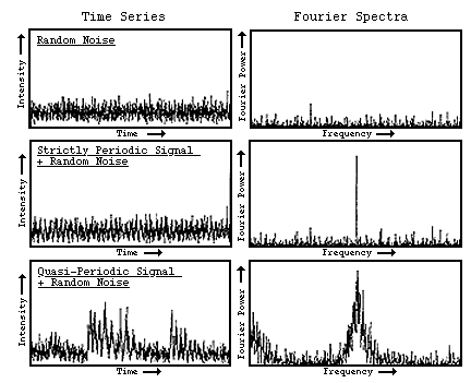
quantitative information. One such quantitative method is Fourier analysis.
Most of you will be aware of the Fourier therom which says that any signal
can be decomposed into an infinite number of sine waves. There are
many tools available which takes an astronomical time series i.e. the light
curve and decomposes it into large number of periodic componnents each with
a different period and a different strength. Very strong components may
appear in data where there is a periodicity present. The plot of the strength
or power of individual component as a function of frequency is known as
Fourier spectrum or Power Density spectrum. Some examples of such power
density spectra are shown in the following figure.
If there is any feature in the power density spectrum indicating additional
power at or around one perticular friquency then one must estimate the significance
of this feature, in other words, to estimate how much confidence one has
in that it represents a true periodicity in the data. When astronomers are
looking for new phenomena, such as pulsars
, they are very conservative in what they take to be a real signal. Power
at any frequency has to be many times more than that would be in a random
data set to be taken seriously.
Another method that is useful for period search is epoch folding.
This is done by chosing a range of periods, and "folding" the data at
those periods. For example, suppose you have a light curve; for 500
seconds with a binsize of 1 second. You want to fold this data on a period
of 25 seconds. To do this, you would start with the first 25 points, and
then add the second 25 points (points 26-50) to the first 25. Now add the
third set of 25 points, and so on, until you reach the end of the data set.
If the period you have chosen has nothing to do with a real period in the
system, then times where the signal is high will cancel out with times where
the signal is low in each of the 25 bins, and the resulting epoch folded
light
curve will look flat and random . If, however, 25 seconds is very close
to the actual period, then bins where the signal is high will add together,
and bins where it is low will add together, and the result will be a very
nice looking epoch folded light curve
. In order to search for exact period one has to first guess a period
and the fold light curve repeatedly around that period to find out exact
period. Once we know the exact period then we can get the folded light curve
at this period. At this point, one must again assess how significant the
resulting light curve is. This is generally done by looking at the spread
of values, or errors, in the typical bin, and comparing how much higher
the values in each bin are than the standard error.
A timing analysis package called XRONOS is available as a part of HEAsoft
. XRONOS includes many independent tasks for: lightcurve(s), hardness ratio
and colour-colour plotting, epoch folding, power spectrum, autocorrelation,
cross-correlation etc. A light curve is generally stored in a FITS file
ending with extension .lc or .flc. Each of the XRONOS tasks
takes these files as an input and gives corrosponding output.
For detail information on timing analysis and XRONOS package please consult
XRONOS User's Guide
. We shall also use some these tasks in our exersises with light curves.
|