Quantum Random Number Generators

Random numbers are the invisible foundation of modern digital security. From generating one-time passwords for online banking and creating encryption keys for secure messaging apps, to ensuring fair outcomes in online games and lotteries, without high-quality randomness, encryption schemes become vulnerable to prediction and attack.

Classical computers cannot produce true randomness. They rely on deterministic algorithms that start from a seed value and follow fixed mathematical rules. The resulting sequence may look random to the human eye (or even pass many statistical tests), but in principle it is completely predictable if the seed and algorithm are known. This is called pseudorandomness. Quantum mechanics, by contrast, is fundamentally probabilistic. The outcome of a quantum measurement is intrinsically unpredictable — not because of incomplete knowledge, but because nature itself does not determine the result in advance. A Quantum Random Number Generator (QRNG) harnesses this intrinsic unpredictability.

However, simply measuring a quantum system is not enough. Hardware imperfections, classical noise, or hidden variables could still influence the outcomes. Our group addresses these challenges by

• 1. testing temporal quantum correlations through the Leggett-Garg Inequality while enforcing the no-signalling-in-time condition
• 2. designing experiments that systematically close major loopholes, and
• 3. mitigate errors from qubit readout, gate imperfections, and classical noise,

ensuring that the generated numbers are certified as truly random by the laws of quantum physics itself.

The Leggett–Garg inequality was introduced to test whether a physical system can be described by a classical picture satisfying two assumptions:

• Macrorealism: a physical system possesses definite properties at all times.
• Non-invasive measurability: those properties can, in principle, be determined without disturbing the subsequent dynamics of the system.

To motivate LGI, let us consider a dichotomic Observable Q, i.e. when measured at any time, it can give two outcomes +1, -1. We can measure Q at three distinct times t₁,t₂,t₃ and build 2-point correlations C_ij as

Note that Q_iQ_j can only have two possible values +1, -1 and consequently C_ij can be atmost 1. For a classical system, (1) can be realized by joint distribution P_ij

Thus the inequality holds even for a classical 2-point function. However, one can go beyond just 2-point function and come up with quantities like

It is easy to see that any instance of K can be atmost 1. This holds for classical system which admits a global distribution P_ijk

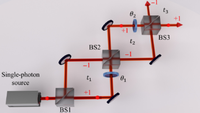
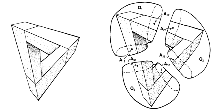
Quantum mechanics, however, permits this bound to be violated for appropriately chosen states, measurements, and time intervals. One can take electronic spin system with Pauli gates as one possible realization of Q. For our case we use the "which path" information of photon in an interferometric setup (see Fig. 1). One can therefore, see that a meaningful global probability distribution P_ijk cannot exist, or, equivalently, one cannot realize the joint distribution P_ij as a marginal of the full distribution. An analogy can be obtained with the help of Penrose's impossible triangle: the object can be broken into units like C₁, C₂, C₃. Although one could glue any pairwise combination of C_i and the resulting diagram would be possible in 3D Euclidean space. There is , however, no consistent way to glue all the units together - much like how there is no consistent way to patch all P_ij's to get P_ijk.