Research highlights

Over the years, I have worked on various problems in the area of statistical physics with an effort to achieve analytical understandings. Some of my research projects along with the main results are highlighted below. For more details about these and other projects [that are not highlighted here], please see the articles listed on the publication page.

Models of active particles

Active particles are self-propelled systems that can generate dissipative, persistent motion by extracting energy from their surroundings at the individual particle level. Examples of active matter can be found in nature at all length scales, ranging from micro-organisms like bacteria to granular matter, a flock of birds, and fish-schools. Even at the level of individual agents (without interactions), active particles show many intriguing features such as non-Boltzmann stationary state [see the figure below] in a confining potential, clustering near the boundaries of the confining region, etc. While the passive counterparts [for example, the Brownian motion] have been studied widely in various contexts, analytical results for active particles are very few. One of our main objectives is to solve simple yet non-trivial models analytically and understand/infer possible useful differences with passive systems.

Run-and-tumble particles (RTP) [see figure 1] and active Brownian particles (ABP) [see figure 2] are the two widely used models for the motion of individual active particles. They describe the overdamped motion of a particle with constant speed along a stochastically evolving internal orientation. For RTP, the internal orientation changes by a finite amount via an intermittent ‘tumbling’ event. On the other hand, the orientation undergoes a rotational diffusion motion for ABP. We have been working on various aspects of active particle dynamics and have obtained various interesting analytical results.

Run and tumble particle (RTP)

1. We have investigated the motion of an RTP in one dimension and found the exact probability distribution of the position with and without diffusion on the infinite line, as well as in a finite interval. We have also analytically studied steady-state as well as the relaxation to the steady-state in a finite domain. We have further computed the survival probability of the RTP in a semi-infinite domain and the exit probability and the associated exit times in the finite interval. ^[1] K. Malakar, V Jemseena, A. Kundu, K Vijay Kumar, S. Sabhapandit, S. N Majumdar, S. Redner, and A. Dhar, J. Stat. Mech. 2018,043215 (2018).
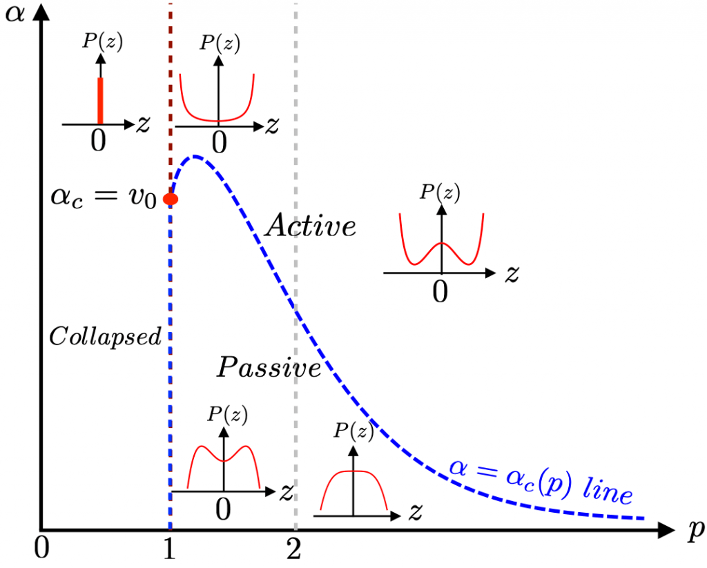
2. We have studied the dynamics of a one-dimensional RTP subjected to confining potentials and found a rather rich behavior for the stationary state probability density, which undergoes a “shape-transition” from an active profile to a passive profile across a critical line in the parameter-space [see figure 4]. We have also studied the full distribution of the first-passage time to the origin analytically. ^[2] A. Dhar, A. Kundu, S. N. Majumdar, S. Sabhapandit, and G. Schehr, Phys. Rev. E 99,032132 (2019).
3. We have studied the motion of a one-dimensional RTP with three discrete internal states in the presence of a harmonic trap of stiffness $\mu$. The three internal states, corresponding to positive, negative, and zero velocities, respectively, evolve following a jump process with a rate $\gamma$. We have computed the stationary position distribution exactly for arbitrary values of $\mu$ and $\gamma$, and show that the distribution undergoes a shape-transition as $\gamma/\mu$ is changed. ^[3]  U. Basu, S. N Majumdar, A. Rosso, S. Sabhapandit, and G. Schehr, J. Phys. A: Math. Theor. 53,09LT01 (2020). 
4. We have studied a set of RTP dynamics in two spatial dimensions, described by how the orientation of the particle changes during tumbling, and calculate exactly the marginal position distributions. ^[4]  I. Santra, U. Basu, and S. Sabhapandit, Phys. Rev. E 101,062120 (2020).
5. We have investigated the run and tumble particle motion in one dimension with position and direction-dependent tumbling rates. For a certain choice of rates, we have found that the particle reaches a stationary state, even in the absence of any external confining potential. We have obtained the exact probability distribution of this non-equilibrium stationary state, as well as studied the approach to the stationary state. We have studied the time-dependent position distribution for cases where there is no stationary state. We have also computed the survival probability in a semi-infinite domain and the exit probability in a finite interval. ^[5] P. Singh, S. Sabhapandit, and A. Kundu, J. Stat. Mech. 2020,083207 (2020). 
6. We have studied the effect of stochastic resetting on an RTP in two spatial dimensions. We compute the radial and $x$-marginal stationary state distributions and show that while the former approaches a constant value as the radial coordinate $r\to 0$, the latter diverges logarithmically as $x\to 0$. On the other hand, both the marginal distributions decay exponentially with the same exponent far away from the origin. We also study the temporal relaxation of the RTP and show that the position distribution undergoes a dynamical transition to a stationary state. We have also studied the first-passage properties of the RTP in the presence of the resetting and show that the optimization of the resetting rate can minimize the mean first passage time. ^[6] I. Santra, U. Basu, and S. Sabhapandit, J. Stat. Mech. 2020, 113206 (2020).

Active Brownian motion with directional reversal

Active Brownian motion with intermittent direction reversals [see figure 3] are common in a class of bacteria like Myxococcus Xanthus and Pseudomonas putida. We show that, for such a motion in two dimensions, the presence of the two time scales set by the rotational diffusion constant $D_R$ and the reversal rate $\gamma$ give rise to four distinct dynamical regimes showing distinct behaviors. We analytically compute the position distribution, which shows a crossover from a strongly non-diffusive and anisotropic behavior at short-times to a diffusive isotropic behavior via an intermediate regime [see the figure below]. We find that the marginal distribution in the intermediate regime shows an exponential or Gaussian behavior depending on whether $\gamma$ is larger or smaller than $D_R$. We also find the persistence exponents in the four regimes. In particular, we show that a novel persistence exponent $\alpha=1$ emerges due to the direction reversal. ^[7]I. Santra, U. Basu, and S. Sabhapandit, arXiv:2101.11327.

Large deviations in nonequilibrium systems

Within the framework of stochastic thermodynamics, the notions of classical thermodynamics such as work, heat and entropy production, etc. can be meaningfully applied to nonequilibrium processes at the level of individual stochastic trajectories of evolution. ^[8]K. Sekimoto, J. Phys. Soc. Japan 66, 1234 (1997); Prog. Theor. Phys. Supp. 130,17 (1998). See also, U. Seifert, Rep. Prog. Phys. 75 126001 (2012) for a review. This framework provides a probabilistic description of the thermodynamic variables for small systems where statistical fluctuations around the average become important [see the figures below]. 

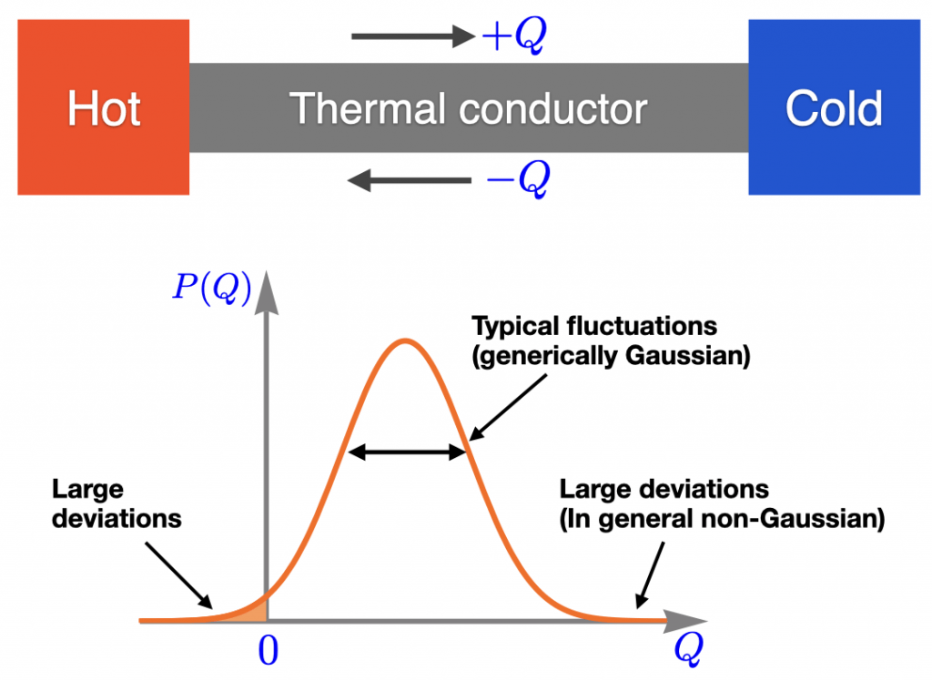
The average quantities satisfy the classical laws of thermodynamics, while the typical fluctuations around the average values are generically Gaussian. However, the large (atypical) fluctuations are not Gaussian, in general. The probabilities of these large fluctuations are generically described by the large deviation form \begin{equation} P(A=a t) \sim e^{-t I(a)},\end{equation} where the observable $A$ may represent the quantities like the heat flow to a system, the work done on a system, the entropy production, etc., in a given time duration $t$. There has been considerable interest in finding the large deviation function [also known as the rate function] $I(a)$, as it encodes the information about the large, atypical, rare fluctuations. In particular, the entropy reducing negative fluctuations [fashionably referred to as the violation of the second-law]—such as the heat flow from a lower temperature to a higher temperature [see figure 6] or the work done on an external force by a system rather than on the system by the force [see the figure below]—fall in this large deviation regime, which tends to zero exponentially with the observation time (or the system size)—recovering the second-law of classical thermodynamics.

Our interest is in the exact calculation of the large deviation probabilities in nonequilibrium systems. We have developed a method for the exact calculation of the large deviation probabilities for one-dimensional systems with harmonic interactions. ^[9] A. Kundu, S. Sabhapandit, and A. Dhar, J. Stat. Mech. 2011,P03007 (2011).

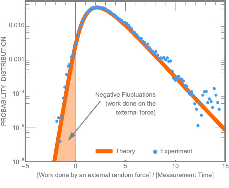
In an experiment carried out by Ciliberto’s group, ^[10]J. R. Gomez-Solano, L. Bellon, A. Petrosyan,  and S. Ciliberto,  EPL 89,  60003 (2010). an AFM micro-cantilever [450 μm long, 50 μm wide and 2 μm thick]—thermalized with the surrounding air—was driven by an external random force [generated by applying a random voltage between the conductive cantilever and a metallic surface brought close to the tip (~10 μm apart)]. The work done by the external force in a given time interval was measured for a large number of realizations, and a probability distribution was constructed. We have analytically calculated the exact large deviation form of the probability distribution. ^[11]S. Sabhapandit, EPL 96,20005 (2011); Phys. Rev. E 85,021108 (2012). Our analytical result is in very good agreement with the experimental findings [see figure 7].

In a second experiment by the same group, a colloidal particle was trapped in an optical trap, and an external force is applied to the particle by modulating the trap position in a correlated random fashion. They measured the work done by the trap on the particle for a given time duration for a large number of realizations and obtained its probability distribution. We have again calculated the exact large deviation form of the probability distribution ^[12]A. Pal and S. Sabhapandit, Phys. Rev. E 87,022138 (2013). of the work done for this case.

We have worked on several other problems and obtained analytical results in this area:

• Work fluctuations for a Brownian particle driven by a correlated external random force. ^[13]A. Pal and S. Sabhapandit, Phys. Rev. E 90,052116 (2014).
• Fluctuation theorem for entropy production of a partial system in the weak-coupling limit. ^[14]D. Gupta and S. Sabhapandit, EPL 115,60003 (2016).
• Stochastic efficiency of an isothermal work-to-work converter engine. ^[15]D. Gupta and S. Sabhapandit, Phys. Rev. E 96,042130 (2017).
• Partial entropy production in heat transport. ^[16]D. Gupta and S. Sabhapandit, J. Stat. Mech. 2018,063203 (2018).
• Entropy production for partially observed harmonic systems. ^[17]D. Gupta and S. Sabhapandit, J. Stat. Mech. 2020,013204 (2020).

Random search processes

Stochastic search processes are ubiquitous in nature. These include animals foraging for food, various biochemical reactions such as proteins searching for specific DNA sequences to bind, or sperm cells searching for an oocyte to fertilize. The study of search strategies has generated tremendous interest in the last few years. A particularly interesting class referred to as the intermittent search strategies, ^[18]O. Bénichou, C. Loverdo, M. Moreau, and R. Voituriez, Rev. Mod. Phys. 83, 81 (2011). involve the combination of (1) local steps when the searcher looks for a target and (2) long-range moves during which the searcher does not look for the target but relocates itself to a different territory.  The slow search phase is typically modeled by diffusion or a random walk. The long-range moves may be modeled depending on the specific application.  A particularly simple long-range strategy consists of “resetting” the searcher to a fixed location [say to the initial starting point] with a finite probability or rate depending on whether the dynamics is in discrete time or in continuous time. The rationale behind this strategy is that if one does not succeed in finding the target via short-range diffusion, it is better to “restart” the process, rather than continuing on the short-range moves.

Stochastic processes under resetting

We have explored the effects of resetting on various stochastic processes.

Lévy flights with resetting

We have proposed and solved analytically a new efficient search model where a searcher performs Lévy flights [as opposed to the local diffusive search] but occasionally, at random times, returns to its initial position. We have shown that a search strategy involving Lévy flights becomes more efficient upon switching on an additional resetting (to the initial position) at a constant rate. Our results demonstrate the existence of a novel first-order phase transition of the optimal search parameters. ^[19]L. Kusmierz, S. N. Majumdar, S Sabhapandit, G Schehr, Phys. Rev. Lett. 113,220602 (2014).

Dynamical transition in the temporal relaxation of stochastic processes under resetting

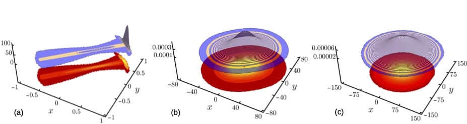
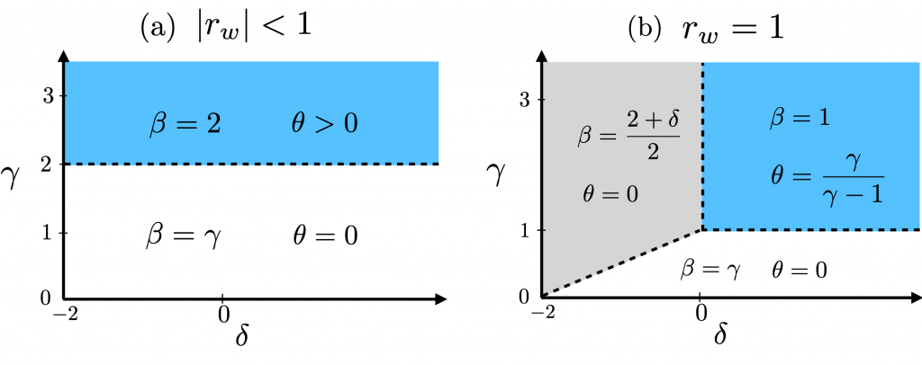
The random resetting leads to nonequilibrium steady states in stochastic processes. We have analytically studied how the steady-state is approached in time and found an unusual relaxation mechanism in these systems:  as time progresses, an inner core region around the resetting point reaches the non-equilibrium steady state (NESS), while the region outside the core is still transient [see the figure below]. ^[20]S. N. Majumdar, S. Sabhapandit, and G. Schehr, Phys.  Phys. Rev. E 91,052131 (2015).

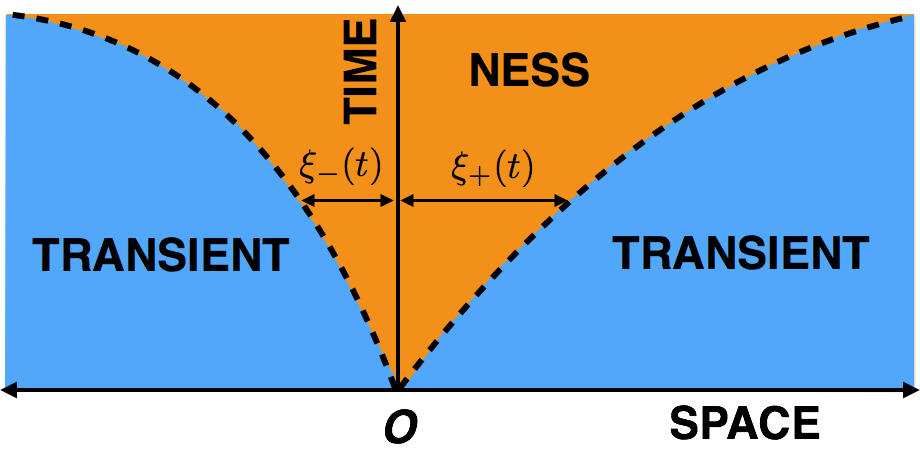
The boundaries of the core region grow with time as power laws at late times with new exponents [see figure 8]. Alternatively, at a fixed spatial point, the system undergoes a dynamical transition from the transient to the steady-state at a characteristic space-dependent timescale $t^*(x)$. The relaxation towards the non-equilibrium steady state (NESS) can be described by a large deviation function that generically exhibits a second-order discontinuity at a pair of critical points characterizing the edges of the inner core. These singularities act as separatrices between typical and atypical trajectories. 

Random walk with random resetting to the maximum position

In an article ^[21]S. N. Majumdar, S. Sabhapandit, and G. Schehr,  Phys. Rev. E 92,052126 (2015).  that received “Editors’ Suggestion“, we have analytically studied a model where the random searcher [modeled by a symmetric random walk on a one-dimensional lattice] remembers the maximum location visited so far and the long-range move consists of resetting to this current maximum [which itself is random]. This strategy may be thought of as a combination of the systematic search and the random search. Since each location is visited only once in the systematic search strategy, if a target in an already visited place is missed [by an imperfect searcher], it is never going to be detected. In our new strategy, the searcher revisits already searched locations [with a certain probability] but also feels a dynamical bias towards exploring new locations [by resetting to the maximum].

Cover times of random walks

A crucial observable to characterize the efficiency of a stochastic search process in a confined region in the important situation where the search process requires an exhaustive exploration of the entire domain, is the so-called cover time $t_c$. This is the minimum time needed such that each point of the entire domain is visited at least once [by at least one of the searchers in case of multiple searchers]. 

Because of its numerous applications—not only for search processes but also in computer science, e.g., in algorithms generating random spanning trees with uniform probability—the statistics of the cover time of stochastic processes have been widely studied [in physics, mathematics, and computer science literature]. However, most of the existing results are restricted to the mean cover time. Obtaining analytical results for the full distribution of $t_c$ is a notoriously hard task—the only exception being the transient walks, ^[22]a random walker that escapes to infinity with a non-zero probability in the unbounded domain where the distribution of [appropriately centered and scaled] $t_c$ approaches a Gumbel distribution, irrespective of the topology of the graph as well as its boundary conditions. ^[23] D. Belius, Probab. Theory Relat. Fields 157, 635 (2013); L. Turban, J. Phys. A: Math. Theor. 48, 445001 (2015); M. Chupeau, O. Bénichou, and R. Voituriez, Nat. Phys. 11, 844 (2015).

The full statistics of the cover time in low dimensions ($d \le 2$), where the random walk is not transient but recurrent, ^[24]starting from a given site, the random walk comes back to it with probability one had been a challenging open question.  We solved ^[25]S. N. Majumdar, S. Sabhapandit, and G.  Schehr,  Phys. Rev. E 94,062131 (2016). this problem for the case of not just one walker, but a more general problem involving a set of $N$ independent one-dimensional Brownian motions [which describe random walks in the long time diffusive scaling limit] on a finite interval, and with different boundary conditions (with reflecting and periodic).

Driven inelastic/granular gasses

It is well-known that a gas of particles undergoing elastic collisions evolves to an equilibrium state where the single-particle velocity distribution is Gaussian [Maxwell distribution]. For such an isolated system, the collisions merely distribute energy among the particles while keeping the total energy constant.

In contrast, if the collisions between particles are inelastic [as in the case of granular matter], the system dissipates energy upon collisions. Without a supply of energy from outside, such systems come to rest in a short time, as we observe in everyday life, like when dropping a marble ball on the floor or while playing billiard. When energy injected from outside compensates for the energy loss due to inelastic collisions, one expects an “inelastic gas” to reach a nonequilibrium steady-state.

What is the velocity distribution for a collection of inelastic particles that is driven to a steady-state through continuous injection of energy and dissipative collisions?

This is the central question in the kinetic theory for dilute inelastic gases, which is widely used in developing phenomenological models for driven granular systems.

Within the kinetic theory, which ignores correlations between pre-collision velocities [molecular chaos hypothesis], for homogeneous, isotropic heating through a thermal bath, the tail of the velocity distribution is a stretched exponential \begin{equation}P(v) \sim \exp\bigl(-a|v|^\beta\bigr)\label{vel-dist-inel-gas}\end{equation} with a universal exponent $\beta=3/2$. ^[26] T. van Noije and M. Ernst, Granular Matter 1, 57 (1998). This result is counterintuitive as it implies that larger speeds are more probable in inelastic systems than the corresponding elastic system with the same mean energy. A derivation of the kinetic theory result, starting from a microscopic model is lacking. In addition, experiments and large-scale simulations are unable to unambiguously determine the tails of the distribution, and hence, a convincing answer to the question is still lacking. 

Using exact analysis, we have investigated the velocity distribution of a driven granular gas starting from microscopic models. Inspired by the collision of particles with a vibrating wall, we have introduced a model for homogeneous driving, where in addition to the interparticle inelastic collisions, the velocity of each particle independently changes at a constant rate according to ^[27]V. V. Prasad, S. Sabhapandit, and A. Dhar, Europhy. Lett. 104,54003 (2013);  Phys. Rev. E 90,062130 (2014). \begin{equation}\boldsymbol{v} \to -r_w\boldsymbol{v} +\boldsymbol{\eta}\quad \text{where} ~~ |r_w| \le 1, \end{equation} and $\boldsymbol{\eta}$ is uncorrelated noise.This model includes both diffusive driving $(r_w=-1)$ and the scenario described by kinetic theory $(r_w=1)$ as special cases.

For generic physically relevant driving, we find ^[28] V V Prasad, D. Das, S. Sabhapandit, and R Rajesh, J. Stat. Mech. 2019,063201 (2019);  Phys. Rev. E 95,032909 (2017); V. V. Prasad, S. Sabhapandit, and A. Dhar, Europhy. Lett. 104,54003 (2013);  Phys. Rev. E 90,062130 (2014). that the tail of the velocity distribution is a Gaussian ($\beta=2$), albeit with additional logarithmic corrections. Thus, the velocity distribution decays faster than the corresponding equilibrium gas. In a less generic second universal regime that corresponds to the scenario described by the kinetic theory, the velocity distribution decays exponentially $(\beta=1)$, with additional logarithmic corrections—in contradiction to the predictions of the phenomenological kinetic theory, necessitating a re-examination of its basic assumptions. See figure 9 for a summary of the results.

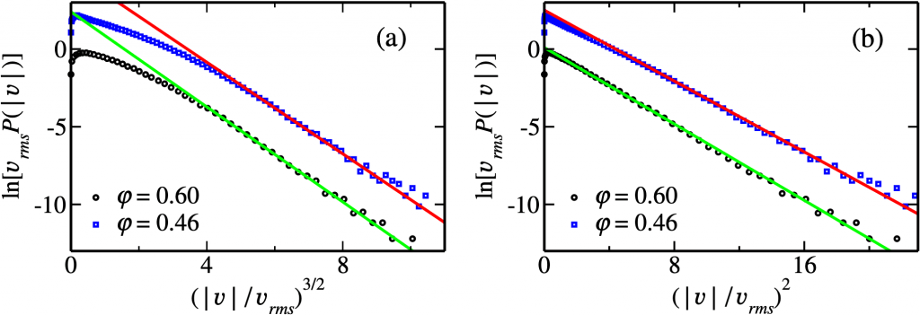
 The experimental data for the measurement of $P(\boldsymbol{v})$ may be open to interpretation. As an example, by re-plotting, we show that the data obtained in a recent experiment with homogeneous driving [see figure 10] and has been argued for evidence for $\beta=3/2$, are also consistent with $\beta=2$. Although the experiment is clearly more complicated than our model, our simulations would suggest that the results are not sensitive to how the system is driven, rather it depends only on whether there is dissipation when particles collide with the wall. In this case, we expect the experiment to fall into the category of $0<r_w<1$, and hence $\beta=2$.

Tagged particle in single-file motion

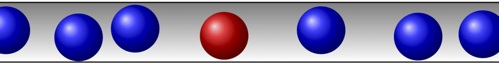
The single-file motion—the motion of particles in narrow channels where the particles cannot pass each other—is a paradigmatic example of movement in a crowded environment [see figure 11]. It has practical implications in diverse systems ranging from transport in biological cells, the motion of colloidal particles in confined geometries, and the motion of atoms and ions in nano-channels. In the single-file motion, the motion of individual particles is hindered by neighboring particles, resulting in a slower motion for individual (tagged) particles. For example, if the individual particle moves ballistically—i.e., moves with a constant velocity—in-between collisions with the neighboring particles, a tagged particle motion is diffusive, ^[30]D. W. Jepsen, J. Math. Phys. (N.Y.) 6, 405 (1965). with the mean square displacement growing linearly with time. On the other hand, for a collection of Brownian particles, a tagged particle shows subdiffusion, ^[31]T. E. Harris, J. Appl. Probab. 2, 323 (1965). with the mean square displacement growing as the square root of the time. While the typical fluctuations are described by Gaussian distribution, the large fluctuations are quite nontrivial.

Universal large deviations for the tagged particle displacement

Consider a gas of point particles distributed with a uniform density $\rho$, moving in a one-dimensional channel with a hardcore interparticle interaction that prevents particle crossings. For an individual particle—in the absence of other particles— we consider a generic propagator \begin{equation}
G(y,t|x,0)= \frac{1}{\sigma_t}\,f\left(\frac{y-x}{\sigma_t}\right),
\label{propagator} 
\end{equation} where $f(-w)=f(w) \ge 0$ and $\int_{-\infty}^\infty |w| f(w)\, dw=\Delta$ is finite. Also, $\int_{-\infty}^\infty f(w)\, dw=1$ due to normalization. We show that the probability distribution of the displacement $X$ in time $t$, of the tagged particle in the single-file motion, has the large deviation form \begin{equation}P_\mathrm{tag}(X,t) \sim \exp\bigl[-\rho \sigma_t I(X/\sigma_t)\bigr],\label{LDform}\end{equation} where the large deviation function is given exactly by \begin{equation}I(z)=2 Q(z)-\bigl[4 Q^2(z)-z^2\bigr]^{1/2},\label{Iz}\end{equation}with\begin{equation}Q(z)= z\int_0^z f(w)\, dw + \int_z^\infty w f(w)\, dw.\label{Qz}\end{equation}

Both for the Brownian particles, as well as for particles moving with the Hamiltonian dynamics with initial velocities chosen independently from Gaussian distribution, the single-particle propagator is Gaussian: $f(w)=\exp(-w^2/2)/\sqrt{2\pi}$ in equation \eqref{propagator} with $\sigma_t \propto \sqrt{t}$ and $\sigma_t \propto t$ respectively for the Brownian and Hamiltonian dynamics. In this case, $Q(z)$ in equation \eqref{Qz} is explicitly given by \begin{equation}Q(z)=\frac{e^{-z^2/2}}{\sqrt{2\pi}}  +\frac{z}{2}\,\mathrm{erf}\bigl(z/\sqrt{2}\bigr).\label{Qz-for-Gaussian}\end{equation}

We have also obtained the cumulant generating function for the generic case, and the first few cumulants for the Gaussian single-particle propagator. See ^[32]C. Hegde, S. Sabhapandit, and A. Dhar, Phys. Rev. Lett. 113,120601 (2014). for details.

Two-tag displacement in single-file motion

We observe the displacement of a tagged particle at time $t$, with respect to the initial position of another tagged particle, such that their tags differ by $r$. Evidently, $r = 0$ corresponds to the case discussed above. We have obtained the exact probability distribution for the two-tagged particle displacement for all times, for general single particle dynamics. As by-products, the large deviation form of the probability distribution is given by \begin{equation} P_\text{tag}(X=\sigma_t z,r=\rho\sigma_tl,t) \sim \exp\bigl[-\rho\sigma_t I_l(z)\bigr], \label{twotag-prob}\end{equation} with \begin{equation}\mspace{-40mu} I_l(z)=2Q(z)-\sqrt{l^2+4Q^2(z)-z^2} +l\ln \left[\frac{l+\sqrt{l^2+4Q^2(z)-z^2}}{2Q(z)+z}\right],\label{twotag-Iz} \end{equation} where $Q(z)$ is still given by equation \eqref{Qz}. One gets back equation \eqref{Iz} by putting $l=0$ in \eqref{twotag-Iz}.

We have again calculated the cumulant generating function and subsequently the first few cumulants for the two-tag case. As a spin-off of our calculation, we also obtain the velocity auto-correlation function,\begin{equation} \frac{1}{\bar{v}^2}\, \bigl\langle v_0(0) v_r(t)\bigr\rangle \simeq \frac{1}{\rho \bar{v} t} \left(\frac{r}{\rho\bar{v} t} \right)^2 f\left(\frac{r}{\rho\bar{v} t}\right),\end{equation}  for the Hamiltonian model of elastically colliding particles, with initial velocities independently are drawn from the distribution ${\bar{v}}^{-1}f(v/\bar{v})$. See ^[33]S. Sabhapandit and A. Dhar, J. Stat. Mech. 2015,P07024 (2015). for details.

Tagged particle diffusion for Hamiltonian dynamics

We have also obtained various spatio-temporal correlation functions of a tagged particle in one-dimensional systems of interacting point particles evolving with Hamiltonian dynamics. See the references ^[34]A. Roy, O. Narayan, A. Dhar, and S. Sabhapandit, J. Stat. Phys. 150,851 (2013) and J. Stat. Phys. 160,73 (2015); A. Kundu, A. Dhar, and S. Sabhapandit, J. Stat. Mech. 2020,023205 (2020).  for details.

Statistics of the front particle (leader) in single-file motion

We have studied the behavior of the leader (rightmost particle) for a semi-infinite system of single-file diffusion, initially distributed in $(-\infty,0)$ with a uniform density $\rho$. See ^[35]S. Sabhapandit, J. Stat. Mech. 2007,L05002 (2007). for details.

Propagator

We find that, starting at the origin, the position of the leader at a later time $t$ is distributed according to the cumulative probability distribution \begin{equation}P(x,t):=\mathrm{Prob}[ \text{leader position} < x] =F\left(\frac{x}{\sqrt{4 D t}},t\right),\end{equation} where the scaling function is given by\begin{equation}F(u,t)=\left[1-\frac{\mathrm{erfc}(u)}{2}\right]\exp\left(-\frac{\rho\sqrt{D t}}{\sqrt{\pi}}\, S(u) \right),\end{equation} with \begin{equation}S(u)=\exp(-u^2) -\sqrt{\pi}\,u\,\mathrm{erfc}(u).\label{Su}\end{equation} At large times, the typical position of the leader grows with time as \begin{equation} a(t)\sim\sqrt{\ln\bigl[\rho \sqrt{D t}/(2\sqrt{\pi})\bigr]}. \label{at}\end{equation} The fluctuation around $a(t)$ at the scale of \begin{equation} b(t)\sim \left[2\sqrt{\ln\bigl[\rho \sqrt{D t}/(2\sqrt{\pi})\bigr]} \right]^{-1}\end{equation} is given by the Fisher-Tippett-Gumbel distribution: \begin{equation} F(u,t) \approx G\left( u-a(t)\over b(t)\right)~~\text{where}~~G(w) = \exp(-\exp(-w)).\label{Gumbel}\end{equation} An equivalent limiting result [given in equation \eqref{Gumbel}] was also obtained earlier by Arratia ^[36] R. Arratia, Ann.  Probab. 11, 362 (1983). in the context of simple symmetric exclusion process.

Maximum position of the leader in a given duration

We find the probability that the leader does not cross the position $z$ ($z\ge 0$), up to time $t$ as \begin{equation}Q(z,t)=\Omega\left(\frac{z}{\sqrt{4 D t}},t\right), \end{equation} where \begin{equation}\Omega(u,t)=\mathrm{erf}(u)\:\exp\left(-\frac{2\rho\sqrt{D t}}{\sqrt{\pi}}\, S(u) \right),\end{equation} with $S(u)$ given in \eqref{Su}. At large times, the fluctuation of the maximum at the scale of \begin{equation} b_m(t)\sim \left[2\sqrt{\ln\bigl[\rho \sqrt{D t}/\sqrt{\pi}\bigr]} \right]^{-1}\end{equation} around \begin{equation} a_m(t)\sim\sqrt{\ln\bigl[\rho \sqrt{D t}/\sqrt{\pi}\bigr]}, \end{equation} is again given by the Fisher-Tippett-Gumbel distribution $G(w)$ given in \eqref{Gumbel}, \begin{equation}\Omega(u,t)\approx G\bigl([u-a_m(t)]/b_m(t)\bigr).\end{equation}

First-passage time

We find the probability density function of the time $\tau$ at which the leader crosses a specified position $z$ for the first time [hence the name first-passage time] as $p_{\text{F}}(\tau,z) = A(\tau,z)\: \exp\bigl(-\Upsilon(\tau,z)\bigr),$ where \begin{align}&A(\tau,z)= \frac{z}{\sqrt{4 \pi D}\, \tau^{3/2}} +\frac{\rho\sqrt{D}}{\sqrt{\pi \tau}}\,\mathrm{erf}\left(\frac{z}{\sqrt{4 D \tau}}\right),\\&\Upsilon(\tau,z)=\frac{z^2}{4 D \tau} +\frac{2\rho\sqrt{D\tau}}{\sqrt{\pi}}\,S\left(\frac{z}{\sqrt{4 D \tau}}\right),\end{align} with $S(u)$ given in \eqref{Su}. In contrast to the $\tau^{-3/2}$ power-law tail for a single diffusing particle [which is reproduced in the limit $\rho=0$], for the leader in the single-file diffusion, the long time asymptotic behavior of the first-passge time distribution is dominated by the stretched-exponential tail $p_{\text{F}}(\tau,z)\sim \exp(-2\rho\sqrt{D\tau}/\sqrt{\pi})$.

Gap and the density profile

How far away is the leader from the rest of the gang? — We investigate this question by considering two measures (i) the gap between the position of the leader to that of the closest particle $\epsilon(t)=x_0(t)-x_1(t)$, and (ii) the density profile with respect to the leader.

We find that, at long times, the gap is distributed exponentially with an effective density of particles near the leader \begin{equation} \Psi_0(\epsilon,t)\sim\exp\bigl(-\overline{\rho}_0(t)\, \epsilon\bigr) ~~\text{with}~~\overline{\rho}_0(t) =\left[\frac{\ln \bigl(\rho\sqrt{Dt}\big/2\sqrt{\pi}\bigr)}{D t} \right]^{1/2}.\label{rho_0}\end{equation}

The density of particles at a distance $\ell$ away from the position of the leader, at long times, is given by \begin{equation}\overline{\rho}(\ell,t)\approx \frac{\rho}{2}\;\mathrm{erfc}\left(a(t)-\frac{\ell}{\sqrt{4 D t}}\right),\end{equation} where $a(t)$ is given in \eqref{at}.

Extremes and Records statistics

Extreme value statistics

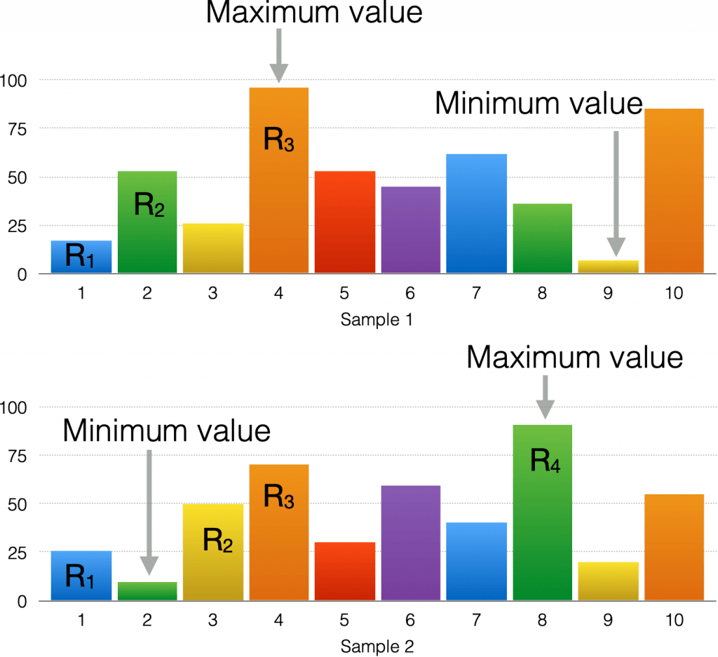
Understanding the statistics of the maximum or the minimum value of a set of random observations [see figure 12] is important in diverse disciplines such as physics, engineering, computer science, finance, hydrology, and atmospheric sciences. For uncorrelated random variables, the statistics of the extreme events is governed by one of the three well-known limit laws: (a) Fréchet, (b) Gumbel, or (c) Weibull, depending on whether the tail of the parent distribution of the random variables, is (a) power law, (b) faster than any power law but unbounded, or (c) bounded, respectively. See these pedagogical lecture notes ^[37]S. Sabhapandit, Extremes and Records,  arXiv:1907.00944. for an introduction. However, much less is understood for systems with strong correlations. We have studied the extremal statistics for a strongly correlated system, namely, the one-dimensional Coulomb gas.

Extremal statistics in the classical 1D Coulomb gas

The set of eigenvalues of a random matrix of independently chosen entries has emerged as the paradigm for strongly correlated random variables. In this context, the Tracy-Widom (TW) distribution for the largest eigenvalue of the Gaussian random matrix has generated a lot of interest for its ubiquity in diverse systems.

For Gaussian ensembles in random matrix theory, the joint probability distribution function of the real eigenvalues can be interpreted as the equilibrium Gibbs distribution of a gas of charges, confined on a line in the presence of an external harmonic potential and repelling each other via two-dimensional logarithmic Coulomb interactions. This system is known as Dyson’s log gas. Interestingly, even though the TW distribution was derived originally for a harmonic confining potential, it has been shown to be universal with respect to the shape of the confining potential, as long as the average charge (eigenvalue) density has a finite support and the density vanishes at the upper edge as a square root. ^[38]P. Bourgade, L. Erdös, H. T. Yau, Commun. Math. Phys. 332, 261 (2014). A natural question then arises whether the TW distribution is robust when one changes, instead of the confining potential, the nature of the repulsive interaction between the charges.

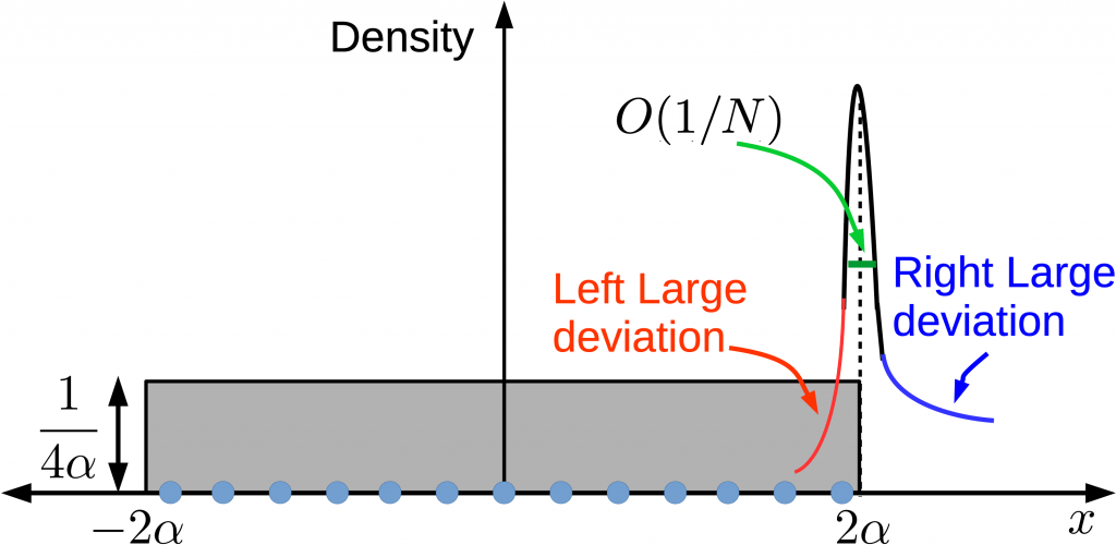
A natural candidate model to address this question is the system of one-dimensional (1D) charges in a harmonic potential but interacting pairwise via the true 1D Coulomb potential. The total energy of the system is given by \begin{equation}\beta\,E(\{x_i\})={N^2\over 2} \sum_{i=1}^N x_i^2 – \alpha N \sum_{i\not= j}|x_i-x_j| \quad\text{with}~~\alpha >0\, .\end{equation} We find the statistics of the position of the rightmost charge. In particular, we find that the typical fluctuation of $O(1/N)$ are described by the probability density function $F’_\alpha(x)$ [analogous to the TW distribution for the Dyson’s log gas], where the cumulative distribution satisfies a nonlocal eigenvalue equation \begin{equation}{dF_\alpha(x)\over dx} = A(\alpha)\,e^{-x^2/2} F_\alpha(x+4\alpha)\label{F-alpha} \end{equation} with the boundary conditions $F_\alpha(-\infty)=0$ and $F_\alpha(\infty)=1$. We also compute the large deviation tails for the atypical fluctuations of $O(1)$, both to the left and to the right of the mean. See ^[39]A. Dhar, A. Kundu, S. N. Majumdar, S. Sabhapandit, and G. Schehr, Phys. Rev. Lett. 119,060601 (2017). for details.

We also study the gap between the two rightmost particles as well as the index—the number of particles on the positive semi-axis. We compute the limiting distributions associated with the typical fluctuations of these observables as well as the corresponding large deviation functions. ^[40] A. Dhar, A. Kundu, S. N Majumdar, S. Sabhapandit, and G. Schehr, J. Phys. A: Math. Theor. 51,295001 (2018). 

Density of near-extreme events

While extreme value statistics is very important, an equally important issue concerns the near-extreme events, i.e., how many events occur with their values near the extreme? In other words, the issue is whether the global maximum (or minimum) value is very far from others [is it lonely at the top?], or whether there are many other events whose values are close to the maximum value. This issue of the crowding of near-extreme events arises in many problems. For instance, in disordered systems, the low-temperature properties are governed by the spectral density function of the excited states near the ground state. In the study of weather and climate extremes, an important question is ‘‘How often do extreme temperature events such as heat waves and cold waves occur?’’ While for an insurance company it is very important to safeguard itself against excessively large claims, it is equally or maybe more important to guard itself against an unexpectedly high number of them. In many of the optimization problems finding the exact optimal solution is extremely hard and the only practical solutions available are the near-optimal ones. In these situations, prior knowledge about the crowding of the solutions near the optimal one is very much desirable.

In this context, we studied quantitatively the phenomenon of the crowding of events near the extreme value for independent random variables and find rather rich and often universal behavior. ^[41]S. Sabhapandit and S. N. Majumdar,  Phys. Rev. Lett. 98,140201 (2007). In fact, by comparing the near-maximum crowding in the reconstructed summer temperature data of western Siberia against the prediction from the independent random variables, we find satisfactory agreement. We also applied this idea to analyze the data from several major international marathons that attract world-class entrants. ^[42]S. Sabhapandit, S. N. Majumdar, and S. Redner,  J. Stat. Mech. 2008,L03001 (2008).

Records statistics

An observation in a time series is called an upper record if its value exceeds that of all previous observations [see figure 12]. Applications of records are found in diverse fields such as meteorology, hydrology, economics, and sports. The study of records has been also useful in understanding and analyzing evolutions in complex systems, ranging from phase slip in charge density waves, ageing in glassy systems, to biological macroevolution and adaptation.

Frequently asked questions in the study of records include

1. How many records occur in a given duration? [number]
2. How long does a record stay before it is broken by a new one? [age]

For a sequence of $N$ independent and identically distributed random variables, the mean number of records $\sim \ln N$ for large $N$, and the typical fluctuations of $O(\sqrt{\ln N})$ around the mean are described by Gaussian distribution. The average age of a record $\sim N/\ln N$ for large $N$. ^[43]See the introductory lectures in S. Sabhapandit, Extremes and Records,  arXiv:1907.00944.

Record statistics of continuous timerandom walk.—There are very few studies on the record statistics for correlated entries. In this context, we have studied the statistics of records for a time series generated by a continuous time random walk and found rather rich behavior. ^[44]S. Sabhapandit, Europhy. Lett. 94,20003 (2011). The results are independent of the details of the jump distribution, as long as it is symmetric and continuous, due to the Sparre-Andersen theorem. ^[45] E. Sparre Andersen, Math. Scand. 1, 263 (1953); 2, 195 (1954); W. Feller, An Introduction to Probability Theory and Its Applications (Wiley, New York, 1968).

We find that the mean number of records $\sim t^{\alpha/2}$ with the observation time $t$, where $\alpha \le 1$:

1. $\alpha=1$ if the mean of the waiting time between two successive jumps is finite. This is true for any waiting time distribution $\rho(\tau)$ that decays faster than the power-law $\tau^{-2}$ tail.
2. For a power-law tail $\rho(\tau) \sim \tau^{-(1+\alpha)}$ of the waiting time distribution with $\alpha<1$, the mean does not exist.

We also find the scaling form of the probability distribution of having $M$ record in time $t$, \begin{equation} P(M,t) \to t^{-\alpha/2} g_\alpha(M t^{-\alpha/2}).\end{equation} The scaling function is given by\begin{equation}g_\alpha(x)=(2/\alpha) x^{-(1+2/\alpha)} L_{\alpha/2}(x^{-2/\alpha}), \quad 0<\alpha\le 1,\end{equation} where $L_\mu(x)$ is the one-sided ($\beta=+1$) Lévy stable probability density function. 

We also study statistics related to the age of records.

Integer partitions and limit shapes

A partition of a positive integer $E$ is a decomposition of $E$ as a sum of a nonincreasing sequence of positive integers $\{h_j\}$: \begin{equation}E=\sum_j h_j \quad\text{such that} \quad h_j \ge h_{j+1}, ~~\text{for}~~ j=1,2\ldots.\end{equation}  For example, the integer $4$ can be partitioned in $5$ different ways: \begin{align*} &4 \\ &3+1\\ &2+2\\ &2+1+1\\&1+1+1+1 \end{align*}

The number of partitions $\rho(E)$ grows with the integer $E$. For example, $\rho(4)=5$ [as illustrated above], $\rho(5)=7$, $\rho(10)=42$, $\rho(100)=190569292$, and so on. Hardy and Ramanujan proved ^[46]G. H. Hardy and S. Ramanujan, Proc. London. Math. Soc. 17, 75 (1918). that for large $E$, the number of partitions grows as \begin{equation} \rho(E) \sim {1\over 4\sqrt{3}\, E} \exp\left(\pi \sqrt{{2E\over 3}}\right)\quad\text{as}~~E\to\infty.\end{equation}

Partitions can be pictorially represented by Young diagrams [also called Ferrers diagrams], where $h_j$ corresponds to the height of the $j$-th column [see the figure below].

In the Young diagram of a given partition of $E$, if $n_i$ denotes the number of columns having heights equal to $i$, then clearly $E=\sum_i n_i\epsilon_i$. This can now be interpreted as the total energy of a non-interacting quantum gas of bosons where $\epsilon_i=i$ for $i=1,2,\ldots,\infty$ represent equidistant single particle energy levels and $n_i=0,1,2,\ldots,\infty$ represents the occupation number of the $i$-th level [see figure 14 (b)].

Restricted partitions.— Consider partitioning a positive integer $E$ into distinct integer summands [strictly decreasing sequence of positive integers]: $E=\sum_j h_j$ such that $h_j > h_{j+1}$. For example, the only allowed restricted partitions of 4 are $4$ and $3+1$. This restricted partition problem having strictly decreasing heights in the Young diagrams corresponds to a non-interacting quantum gas of fermions, for which $n_i=0,1$. The number of such restricted partitions grow with $E$ as ^[47]G. E. Andrews, The Theory of Partitions (Cambridge University Press, Cambridge 1998) \begin{equation} \rho(E) \sim {1\over 4 \times 3^{1/4}\, E^{3/4}} \exp\left(\pi \sqrt{{E\over 3}}\right)\quad\text{as}~~E\to\infty.\end{equation}

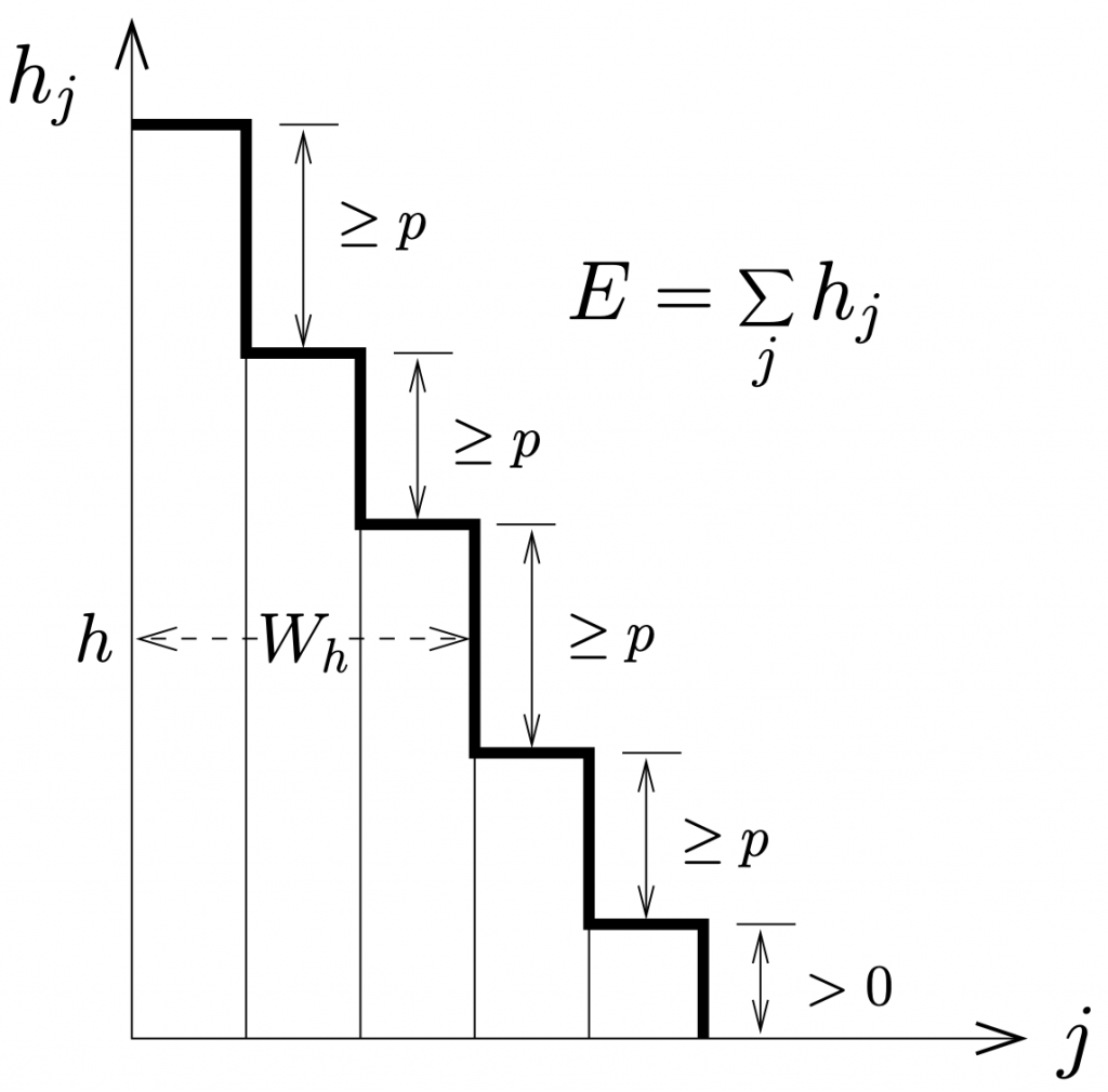
Minimal difference $p$ partition (MDP–$p$).— In the MDP-$p$ problem, a positive integer $E$ is expressed as a sum of positive integers $E=\sum_j h_j$ such that $h_j-h_{j+1}\ge p$ [see the figure below].  Therefore, $p=0$ corresponds to unrestricted partitions and $p=1$ to restricted partitions into distinct parts. 

In terms of the system of quantum particles occupying equidistant energy levels, again for $p>1$ a level can be occupied by at most one particle. However, now the gap between two adjacent occupied energy levels must be at least $p$, i.e., when an energy level is occupied by a particle, the adjacent $p-1$ levels must remain unoccupied. When analytically continued to non-integer values $0<p<1$, it corresponds to a gas of quantum particles obeying fractional exclusion statistics.

Limit shapes

The shape [height profile] of a partition can be defined by the width $W_h$ of the Young diagram at a height $h$ [see figure 15]. In other words, $W_h$ is the number of columns of the Young diagram whose height is greater than or equal to $h$.  In the corresponding quantum system, $W_h$ represents the total number of particles occupying energy levels above $h$.

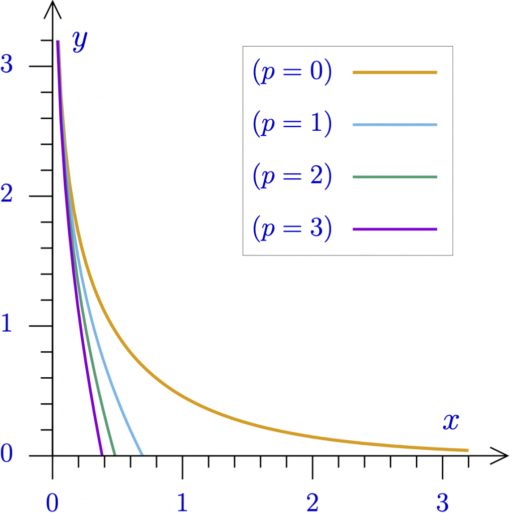
For a partition is randomly chosen with uniform measure from the ensemble of all the partitions of an integer $E$, the curve $W_h/\sqrt E$ as a function of $h/\sqrt E$ converges to a limit curve [i.e., the random variable $W_h/\sqrt{E}$ is strongly peaked around its mean value] when $E\rightarrow\infty$.  We have obtained the limit shapes for MDP-$p$ for general $p$. ^[48]A. Comtet, S. N Majumdar, S. Ouvry, and S. Sabhapandit, J. Stat. Mech. 2007, P10001 (2007); A. Comtet, S. N Majumdar, and S. Sabhapandit, J. Math. Phys. Anal. Geom. 4, 24 (2008). [see equation \eqref{eq-limitshapes} below]

The mathematical expression for the limit shapes.— We define the scaling variables \begin{equation} x={b(p)\,W_h\over \sqrt E}\quad \text{and} \quad y={b(p)\,h\over\sqrt E},\end{equation} where $b(p)$ is a constant which depends on the parameter $p$,\begin{equation}  b^2(p)= \frac{\pi^2}{6} -\mathrm{Li_2} (1/y^*)-\frac{p}{2} (\ln y^*)^2,\label{bp}\end{equation} with $y^*$ being the (only) real positive root of the equation $y^* -y^{* 1-p}=1$, and $\mathrm{Li_2}(z)=\sum_{k=1}^\infty z^k k^{-2}$ being the dilogarithm function. ^[49] See Wikipedia or mathworld

The limit shape is given by the equation \begin{equation} y=- \ln (1-e^{-x}) -px.\label{eq-limitshapes}\end{equation}

Special cases.— (a) For $p=0$ [unrestricted partition], \eqref{bp} gives $b(0)=\pi/\sqrt{6}$ and from \eqref{eq-limitshapes}, the limit shape is given by the equation ^[50]This was first computed by H. N. V. Temperley, Proc. Cambridge Philos. Soc.  48, 683 (1952) \begin{equation} e^{-x} + e^{-y} =1.\end{equation}

(b) For $p=1$ [restricted partition], \eqref{bp} gives $b(1)=\pi/\sqrt{12}$ and \eqref{eq-limitshapes} gives the limit shape as ^[51] It was obtained by Vershik and collaborators: Funct. Anal. Appl. 30, 90 (1996); Theory Probab. Appl. 44, 453 (2000); Moscow Math. J. 1, 457 (2001).  \begin{equation} e^{x}-e^{-y}=1.\end{equation}

Figure 16 shows the limit shapes for $p=0,1,2$, and $3$.

Largest part of Young diagrams

For a partition is randomly chosen with uniform measure from the ensemble of all the partitions of a given integer $E$, we find that the cumulative distribution of the largest height tends to the Gumbel distribution as $E\to\infty$: \begin{equation} \mathrm{Prob}~[h_1 < l] \to F\left(\frac{b(p)}{\sqrt{E}} \Bigl[l-l^*(E) \Bigr]\right),\end{equation} where $F(z)=\exp[-\exp(-z)]$ and $l^*(E) =[\sqrt{E}/b(p)]\ln\bigl[\sqrt{E}/b(p)\bigr]$.