Spectral Analysis: Exercise 1
X-ray spectrum of an Anomalous X-ray Pulsar
This exercise is meant to introduce to you the concept of spectral
analysis by fitting a model for the X-ray spectra of the anomalous X-ray pulsar
4U 0142+61
. In order to analyse the spectra we essentially need two files, the PHA
file(pulse height amplitude, generally with the extension .pha) containing
the count of photons recorded by the detector in each energy channel, and
the response file (generally with the extension .rmf or .rsp) needed
to convolve the model (that we are trying to fit) with the detector response.
Generally the PHA file extracted from the raw date of any particular instrument
/ mission is not corrected for the background, and hence another PHA
file containing the background spectrum (background photon count for each
channel) is needed to
subtract from the source count. In most cases we also need an auxiliary response
file (generally with extension .arf) which contain miscellaneous details
of the instrument response. All this different files are strictly in FITS
format.
The standard software used for analysing the X-ray spectra is
xspec
, which is a part of the
HEAsoft
-
Xanadu
software. The first action to be taken is to copy required source and
background spectrum files,
4U0142_sis0src.pha,
4U0142_sis0bkg.pha
and instrument response files, sis0.arf
and sis0.rmf
.
Now invoke the software by typing xspec at your prompt.
pulsar> xspec
Now supply the name of the source data (PHA) file.
XSPEC>data sis0src.pha
 Net count rate (cts/s) for file  1   5.175    +/-  1.5519E-02
  1 data set is in use
Now provide the rmf, arf file.
XSPEC>resp sis0.rmf
XSPEC>arf sis0.arf
And the background spectrum file.
XSPEC>back sis0bkg.pha
 Net count rate (cts/s) for file   1   5.162    +/-  1.5520E-02( 99.8% total)
   using response (RMF) file...       sis0.rmf
   using auxiliary (ARF) file...      sis0.arf
   using background file...           sis0bkg.pha
While analysing the spectra one needs to repeatedly see the graphical representation
of the spectra, so invoke the graphical display device.
XSPEC>cpd /xw
If your system supports device other than /xw then you may invoke
the particular device of your choice. Now plot the spectra.
XSPEC>plot data
And this is the plot you will see.
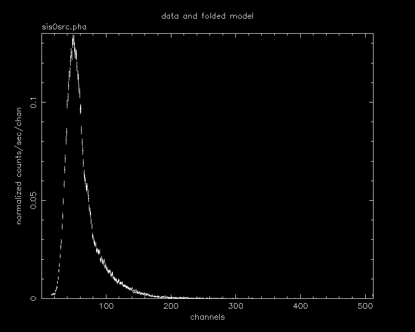
Obviously to glean useful information one needs to view spectra as a function
of energy, rather than as a function of channel nos. of the particular instrument.
So change the unit of x-axis to that of energy (keV).
XSPEC>setplot energy
XSPEC>pl
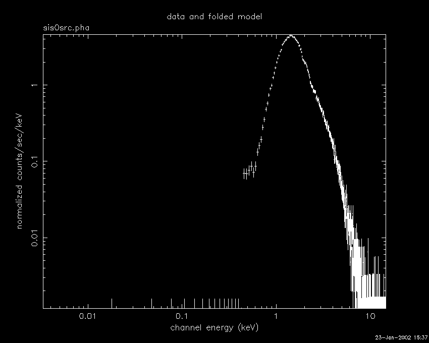
Now one needs to judiciously decide on the channel nos. (energy ranges)
to be included in the analysis and reject the poor quality data. Looking at
the spectra notice that the data below 0.5 keV and above 10.0 keV need to
be excluded.
XSPEC>ignore **-0.5
XSPEC>ignore 10.0-**
It is the normal practice to plot the spectra on a log scale.
XSPEC>pl ldata
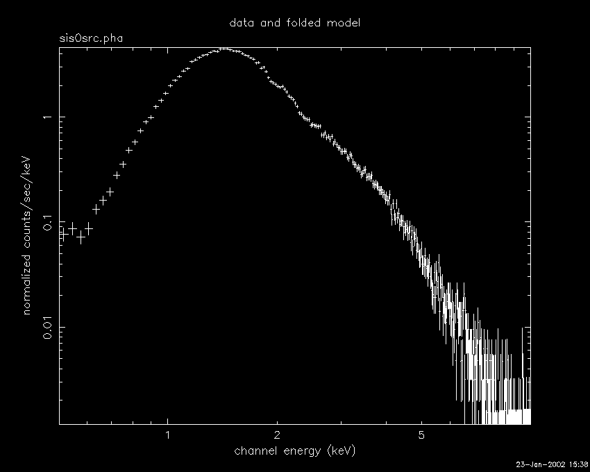
This is now an acceptable sepctra ready for analysis.
Commence to fit spectral model (right now use the ones already available
with the xspec package). Before fitting you might want to go have a
glance at all the models avialble with xspec with their parameters.
XSPEC>help models
...
...
Without wasting precious time now lets get into serious model fitting,
if you want to really know about the various models and their parameters you
have all the time later to browse through them.
From our experience, as the first step, we will ask you to fit the simple
powerlaw model .
XSPEC>model powerlaw
  Model:  powerlaw[1]
Input parameter value, delta, min, bot, top, and max values for ...
Current:           1      0.01        -3        -2         9        10
powerlaw:PhoIndex>1.0
Current:           1      0.01         0         0     1E+24     1E+24
powerlaw:norm>1.0
  ---------------------------------------------------------------------------
  ---------------------------------------------------------------------------
  Model:  powerlaw[1]
  Model Fit Model Component  Parameter  Unit     Value
  par   par comp
    1    1    1   powerlaw   PhoIndex            1.000     +/-   0.000
    2    2    1   powerlaw   norm                1.000     +/-   0.000
  ---------------------------------------------------------------------------
  ---------------------------------------------------------------------------
 Chi-Squared =     7.2227782E+08 using   326 PHA bins.
 Reduced chi-squared =      2229252.     for    324 degrees of freedom
 Null hypothesis probability =  0.00
We gave the arbitrary initial value 1.0 to both the powerlaw parameters,
viz. photon index and the norm. The last three lines give the statistics of
the fit, and one doesn't need to be whiz kid in statistics to realise the
unacceptabilty of the fit by these parameter values. So now give the command
fit to find the parameter values coresponding to the best fit of the
model (powerlaw) with the data.
XSPEC>fit
You'll get some response like this
 Chi-Squared    Lvl  Fit param # 1     2
   64064.7     -1      1.594      1.2661E-02
   63617.6     -2      1.403      1.2501E-02
   63281.0     -3      1.527      1.3237E-02
   63201.4     -4      1.457      1.2675E-02
   63171.9     -5      1.499      1.2961E-02
   63162.2     -6      1.474      1.2780E-02
   63158.6     -7      1.489      1.2883E-02
   63157.4     -8      1.480      1.2820E-02
   63156.9     -9      1.486      1.2857E-02
   63156.8    -10      1.482      1.2835E-02
 Number of trials exceeded - last iteration delta =   0.1602
 Continue fitting? (Y)
Continue fitting till the least chi square value is obtained. The best
fit parameter values and the statistics of the fit will be provided.
Model:  powerlaw[1]
  Model Fit Model Component  Parameter  Unit     Value
  par   par comp
    1    1    1   powerlaw   PhoIndex            1.484     +/-  0.5001E-02
    2    2    1   powerlaw   norm               1.2845E-02 +/-  0.6903E-04
  ---------------------------------------------------------------------------
  ---------------------------------------------------------------------------
 Chi-Squared =      63156.70     using   326 PHA bins.
 Reduced chi-squared =      194.9281     for    324 degrees of freedom
 Null hypothesis probability =  0.00
This fit is also extremely poor. See the spectra, the best fit model and
the residual (difference between the data and the model for each energy bin)
to decide the course of next action.
XSPEC>pl ld residual
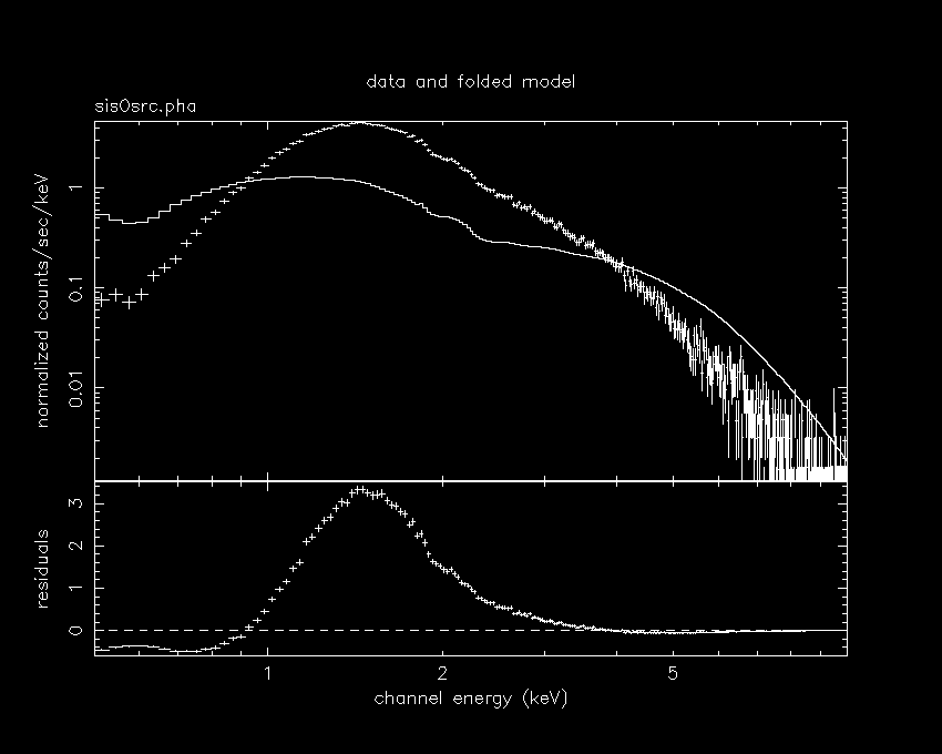
Notice in the spectra that the data is absorbed in the lower end. Hence
introduce another model component for the absorption due to effective Hydrogen
column in the direction of the source.
XSPEC>addcomp 1 wabs
Input parameter value, delta, min, bot, top, and max values for ...
Current:           1     0.001         0         0     1E+05     1E+06
wabs:nH>1.0
  ---------------------------------------------------------------------------
  ---------------------------------------------------------------------------
  Model:  wabs[1]( powerlaw[2] )
  Model Fit Model Component  Parameter  Unit     Value
  par   par comp
    1    3    1   wabs       nH       10^22      1.000     +/-   0.000
    2    1    2   powerlaw   PhoIndex            1.483     +/-  0.5002E-02
    3    2    2   powerlaw   norm               1.2842E-02 +/-  0.6902E-04
  ---------------------------------------------------------------------------
  ---------------------------------------------------------------------------
 Chi-Squared =      82951.66     using   326 PHA bins.
 Reduced chi-squared =      256.8163     for    323 degrees of freedom
 Null hypothesis probability =  0.00
Again fit.
XSPEC>fit
Continue till the least chi-square value is reached.
 ---------------------------------------------------------------------------
  Model:  wabs[1]( powerlaw[2] )
  Model Fit Model Component  Parameter  Unit     Value
  par   par comp
    1    3    1   wabs       nH       10^22      1.466     +/-  0.9978E-02
    2    1    2   powerlaw   PhoIndex            4.122     +/-  0.1642E-01
    3    2    2   powerlaw   norm               0.5542     +/-  0.9438E-02
  ---------------------------------------------------------------------------
  ---------------------------------------------------------------------------
 Chi-Squared =      1086.914     using   326 PHA bins.
 Reduced chi-squared =      3.365060     for    323 degrees of freedom
 Null hypothesis probability =  0.00
The value of (reduced) chi-square has come down, considerably, but still
far from acceptable. Observe the spectra now (give pl command)and notice
the excess in emission. Introduce the model component for blackbody emission
and fit.
XSPEC>addcomp 2 bb
Input parameter value, delta, min, bot, top, and max values for ...
Current:           3      0.01     1E-04      0.01       100       200
bbody:kT>3.0
Current:           1      0.01         0         0     1E+24     1E+24
bbody:norm>1.0
...
XSPEC>fit
...
till you get the least chi-square value. You will get something like this.
Chi-Squared =      1086.914     using   326 PHA bins.
 Reduced chi-squared =      3.386025     for    321 degrees of freedom
 Null hypothesis probability =  0.00
Well, the fit is still unacceptable. The trick is in providing proper
intial values to the parameters and then commence the fitting. Here we will
bail you out by providing the approximately best fit parameter values, please
input the following very carefully,and then fit till the parameter values
converge again to the least chi-square.
XSPEC>newpar 1 1.0
    5 variable fit parameters
 Chi-Squared =      68922.85     using   326 PHA bins.
 Reduced chi-squared =      214.7129     for    321 degrees of freedom
 Null hypothesis probability =  0.00
XSPEC>newpar 2 0.4
    5 variable fit parameters
 Chi-Squared =      151527.9     using   326 PHA bins.
 Reduced chi-squared =      472.0494     for    321 degrees of freedom
 Null hypothesis probability =  0.00
XSPEC>newpar 3 0.001
    5 variable fit parameters
 Chi-Squared =      8851.366     using   326 PHA bins.
 Reduced chi-squared =      27.57435     for    321 degrees of freedom
 Null hypothesis probability =  0.00
XSPEC>newpar 4 3.5
    5 variable fit parameters
 Chi-Squared =      8851.366     using   326 PHA bins.
 Reduced chi-squared =      27.57435     for    321 degrees of freedom
 Null hypothesis probability =  0.00
XSPEC>newpar 5 0.2
    5 variable fit parameters
 Chi-Squared =      70629.30     using   326 PHA bins.
 Reduced chi-squared =      220.0290     for    321 degrees of freedom
 Null hypothesis probability =  0.00
XSPEC>pl
XSPEC>fit
...
...
  ---------------------------------------------------------------------------
  ---------------------------------------------------------------------------
  Model:  wabs[1]( bbody[2] + powerlaw[3] )
  Model Fit Model Component  Parameter  Unit     Value
  par   par comp
    1    1    1   wabs       nH       10^22      1.019     +/-   0.000
    2    2    2   bbody      kT       keV       0.3980     +/-   0.000
    3    3    2   bbody      norm               1.8085E-03 +/-   0.000
    4    4    3   powerlaw   PhoIndex            3.542     +/-   0.000
    5    5    3   powerlaw   norm                0.1553    +/-   0.000
  ---------------------------------------------------------------------------
  ---------------------------------------------------------------------------
 Chi-Squared =      321.8896     using   326 PHA bins.
 Reduced chi-squared =      1.002771     for    321 degrees of freedom
 Null hypothesis probability = 0.476

!XSPEC> statistic chi;
 Chi-Squared =      321.8896     using   326 PHA bins.
 Reduced chi-squared =      1.002771     for    321 degrees of freedom
 Null hypothesis probability = 0.476
Viola!!!! Very well fit! This is definitely a very good model fitting
of the data. Probably the ideal spectral modelling of an anomalous X-ray pulsar.
See the spectra and the residual.
XSPEC>pl ld re
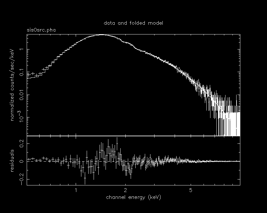
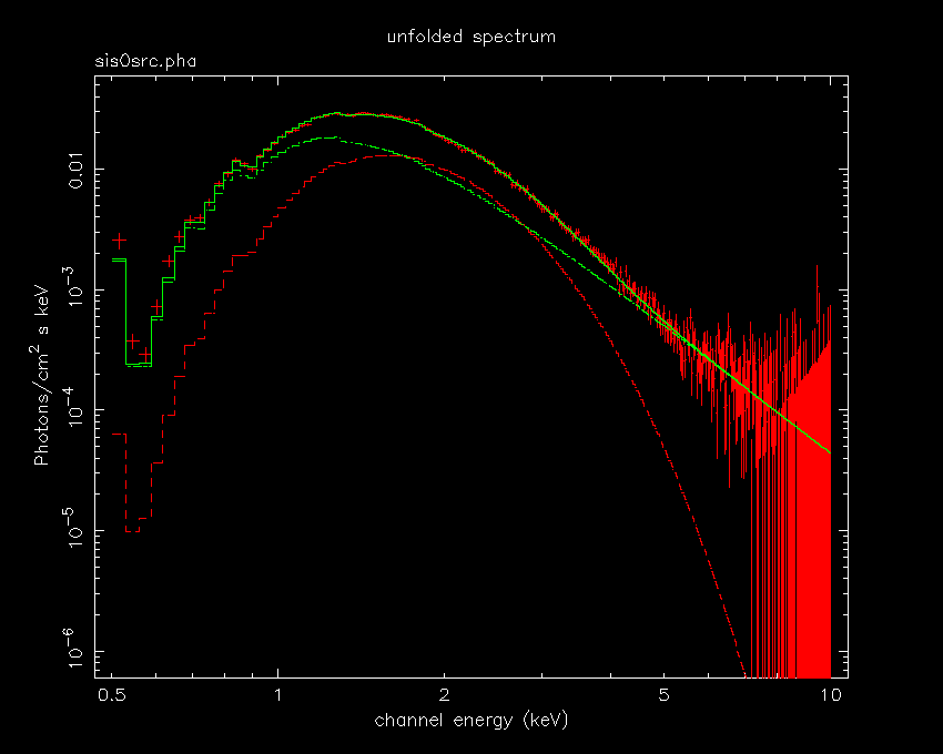
This is what you see. You may also want to see the unfolded sepctra.
XSPEC>pl uf
And see this beautiful spectra with the ideal model fitting the data, along
with the individual model components.
Now quit the xspec pacakge.
XSPEC>quit
The power-law photon index of 3.5 of this pulsar is much larger than the
accreting high mass binary X-ray pulsars and is a feature common to the anomalous
X-ray pulsars. The X-ray luminosity of the black body
component of the spectrum can be estimated if the distance of this pulsar
is known. If the amount of black body flux incident on per unit area
of the detector is F, then the luminosity of the black body component is
L = (4 pi d^2 F), which must also be equal to (pi r^2 sigma T^4), where T
is the temperature of the black body component and r is the radius of the
emission region. T and F are measured from the X-ray spectrum, d is
estimated by studying a supernova remnant associated with this pulsar. The
radius of the emission region (r)
calculated using the above expression is only about a few kilometers. This
suggests that the object must be
a compact star, most probably a neutron star.
So this was the first exercise in spectral analysis of X-ray sources. Our
next step will be to incorporate emission-line spectroscopy along with the
continuum components.
|


