Spectral Analysis: Exercise 3
Fitting multiple lines
In this exercise we will analyse spectrum of the binary X-ray pulsar
Vela X-1
taken during an eclipse. The companion star blocks the X-rays emitted from
regions near the neutron star from reaching us. Hard X-rays from the pulsar
excites the strong outflowing wind of the companion star and this plasma
reemits X-rays which is reach in line emission. We will find that the eclipse
X-ray spectrum of this source contains multiple emission lines (generally
the indication of presence of photoionised plasma). The initial procedures
must be familiar by now, so lets get on with the business quickly, i.e. copy
the required files velax-1_sis01src.pha
, velax-1_sis01src.pha
, sis01.rsp
and start xspec
, invoke the graphical display device, and give the data file. (by the way,
ignore the warnings that follow) .
pulsar>xspec
XSPEC>cpd /xw
XSPEC>setp e
XSPEC>da sis01src.pha
 *WARNING*:  Response and data file telescope ID mismatch
 (ASCA,UNKNOWN) for file   1
 *WARNING*:  Response and data file instrument ID mismatch
 (SIS0,UNKNOWN) for file   1
 Net count rate (cts/s) for file   1  0.2287    +/-  2.2312E-03( 99.0% total)
   using response (RMF) file...       sis01.rsp
   using background file...           sis01bkg.pha
   1 data set is in use
Wow!!! The software this time automatically recognised the response file
and the background file without us provifding it!!! Although it may seem magical,
fortunately or unfortunately the software can't really read your mind and
decide what you need or want unless you tell it . The information about
the response and the background file was already stored in the header
of this source PHA file (refer to FITS file format). Ignore channels below
0.5 keV and above 10.0 keV and see the spectra
XSPEC>ig **-0.5 10.-**
XSPEC>pl ld
and start fitting with powerlaw with an absorption component,
wabs , and fit till the best chi-square value is obtained.
XSPEC>mo wabs po
 MODPRS : Model in the old style syntax was converted to the new syntax:
 mo = wabs((po)).
  Model:  wabs[1]( powerlaw[2] )
Input parameter value, delta, min, bot, top, and max values for ...
Current:           1     0.001         0         0     1E+05     1E+06
wabs:nH>
Current:           1      0.01        -3        -2         9        10
powerlaw:PhoIndex>
Current:           1      0.01         0         0     1E+24     1E+24
powerlaw:norm>
  ---------------------------------------------------------------------------
  ---------------------------------------------------------------------------
  Model:  wabs[1]( powerlaw[2] )
  Model Fit Model Component  Parameter  Unit     Value
  par   par comp
    1    1    1   wabs       nH       10^22      1.000     +/-   0.000
    2    2    2   powerlaw   PhoIndex            1.000     +/-   0.000
    3    3    2   powerlaw   norm                1.000     +/-   0.000
  ---------------------------------------------------------------------------
  ---------------------------------------------------------------------------
 Chi-Squared =     4.6784712E+09 using   206 PHA bins.
 Reduced chi-squared =     2.3046656E+07 for    203 degrees of freedom
 Null hypothesis probability =  0.00
XSPEC>fit
..
..
  ---------------------------------------------------------------------------
  ---------------------------------------------------------------------------
  Model:  wabs[1]( powerlaw[2] )
  Model Fit Model Component  Parameter  Unit     Value
  par   par comp
    1    1    1   wabs       nH       10^22     2.9319E-14 +/-  0.3724E-01
    2    2    2   powerlaw   PhoIndex           0.1686     +/-  0.2859E-01
    3    3    2   powerlaw   norm               4.2354E-04 +/-  0.3118E-04
  ---------------------------------------------------------------------------
  ---------------------------------------------------------------------------
 Chi-Squared =      1048.731     using   206 PHA bins.
 Reduced chi-squared =      5.166165     for    203 degrees of freedom
 Null hypothesis probability =  0.00
Guess you must be aware by now that you don't generally get an acceptable
fit in the first go, so be happy about the chi-square value obtained for the
time being and observe the spectra, best fit model and the residual.
XSPEC>pl ld delc
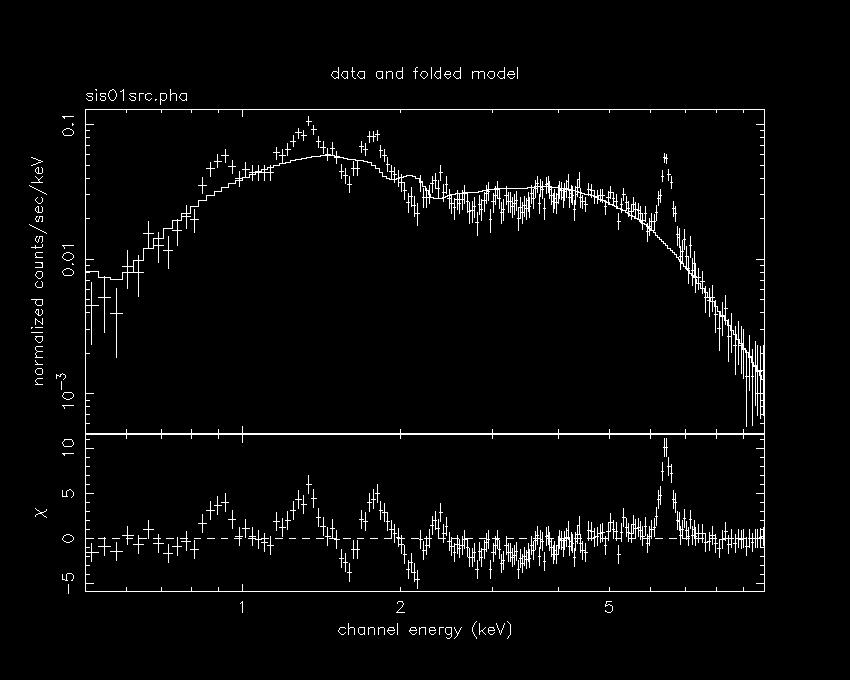
Observe the various emission line elements (especially in the residual).
We have to start fitting them. Introduce a gaussian at 6.4 keV (Fe
emission line) with reasonable intial values of the parameters, especially
the norm (refer to the best fit paramters of the previous exercise)
XSPEC>addcomp 3 ga
Input parameter value, delta, min, bot, top, and max values for ...
Current:         6.5      0.05         0         0     1E+06     1E+06
gaussian:LineE>6.4
Current:         0.1      0.05         0         0        10        20
gaussian:Sigma>0.1
Current:           1      0.01         0         0     1E+24     1E+24
gaussian:norm>5e-4
..
..
XSPEC>fit
..
..
  ---------------------------------------------------------------------------
  ---------------------------------------------------------------------------
  Model:  wabs[1]( powerlaw[2] + gaussian[3] )
  Model Fit Model Component  Parameter  Unit     Value
  par   par comp
    1    1    1   wabs       nH       10^22      0.000     +/-  -1.000
    2    2    2   powerlaw   PhoIndex           0.2498     +/-  0.1899E-01
    3    3    2   powerlaw   norm               4.4656E-04 +/-  0.1808E-04
    4    4    3   gaussian   LineE    keV        6.442     +/-  0.8507E-02
    5    5    3   gaussian   Sigma    keV       0.1051     +/-  0.1355E-01
    6    6    3   gaussian   norm               3.7930E-04 +/-  0.3634E-04
  ---------------------------------------------------------------------------
  ---------------------------------------------------------------------------
 Chi-Squared =      566.9811     using   206 PHA bins.
 Reduced chi-squared =      2.834905     for    200 degrees of freedom
 Null hypothesis probability = 7.911E-37
and see the spectra and residual.
XSPEC>pl
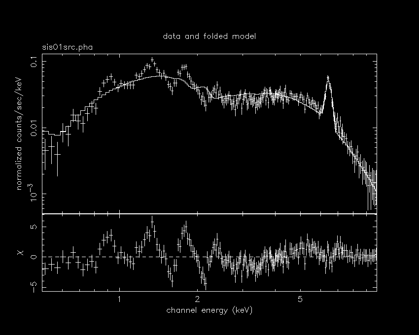
Note that the line at 6.4 keV is no longer there in the residual. Now lets
add another line component, say the one at 1.3 keV, and fit .
XSPEC>addcomp 4 ga
Input parameter value, delta, min, bot, top, and max values for ...
Current:         6.5      0.05         0         0     1E+06     1E+06
gaussian:LineE>1.3
Current:         0.1      0.05         0         0        10        20
gaussian:Sigma>
Current:           1      0.01         0         0     1E+24     1E+24
gaussian:norm>
..
XSPEC>fit
..
..
  ---------------------------------------------------------------------------
  ---------------------------------------------------------------------------
  Model:  wabs[1]( powerlaw[2] + gaussian[3] + gaussian[4] )
  Model Fit Model Component  Parameter  Unit     Value
  par   par comp
    1    1    1   wabs       nH       10^22     0.1116     +/-  0.9912E-01
    2    2    2   powerlaw   PhoIndex          -0.2000     +/-  0.6520E-01
    3    3    2   powerlaw   norm               2.3017E-04 +/-  0.4569E-04
    4    4    3   gaussian   LineE    keV        6.438     +/-  0.8412E-02
    5    5    3   gaussian   Sigma    keV       7.6545E-02 +/-  0.1684E-01
    6    6    3   gaussian   norm               3.3097E-04 +/-  0.3657E-04
    7    7    4   gaussian   LineE    keV       0.2979     +/-   1.270
    8    8    4   gaussian   Sigma    keV       0.9435     +/-  0.5153
    9    9    4   gaussian   norm               1.3220E-03 +/-  0.3739E-02
  ---------------------------------------------------------------------------
  ---------------------------------------------------------------------------
 Chi-Squared =      437.1687     using   206 PHA bins.
 Reduced chi-squared =      2.219131     for    197 degrees of freedom
 Null hypothesis probability = 2.874E-20
Hmmmm... the chi-square value has definitely come down, and the trend shows
that if we add the other lines then perhaps the fit will turn out to be very
good.... but, shouldn't you check the paramter values, and decide whether
they are acceptable or not? Still if you are not yet decided about the acceptability
of the parameter values then see the spectra with its individual components
(prefereably the unfolded sepctra).
XSPEC> pl uf
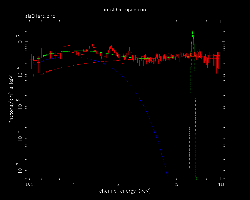
Now it is clear that the line at 1.3 keV is unacceptable with the given
width (sigma = 0.94 keV). Can you guess what has happened? While fitting,
the program has tried to obtain the best fit by incorporating all the lines
(at low energy range) by just one gaussian type emission line function.
This shows that firstly, one should not happily accept any best fit model
just by statistical viability, the model has to be physically and logically
acceptable, and secondly, we should be careful in giving the initial values
of the parameters when we introduce any new model component. There are various
ways of setting the things right, and lets follow the longest but safest
way: delete the last line component.
XSPEC>delc 4
  Model:  wabs[1]( powerlaw[2] + gaussian[3] )
 Chi-Squared =      1425.508     using   206 PHA bins.
 Reduced chi-squared =      7.127539     for    200 degrees of freedom
 Null hypothesis probability =  0.00
Notice the increase in the chi-square value, that is because the values of
these old paramters have changed while we are trying to fit the line at 1.3
keV. So we have to fit again till we get the previous best fit.
XSPEC>fit
..
..
  ---------------------------------------------------------------------------
  ---------------------------------------------------------------------------
  Model:  wabs[1]( powerlaw[2] + gaussian[3] )
  Model Fit Model Component  Parameter  Unit     Value
  par   par comp
    1    1    1   wabs       nH       10^22     1.5959E-12 +/-  0.3764E-01
    2    2    2   powerlaw   PhoIndex           0.2179     +/-  0.3095E-01
    3    3    2   powerlaw   norm               4.2746E-04 +/-  0.3296E-04
    4    4    3   gaussian   LineE    keV        6.442     +/-  0.8504E-02
    5    5    3   gaussian   Sigma    keV       0.1026     +/-  0.1386E-01
    6    6    3   gaussian   norm               3.7504E-04 +/-  0.3673E-04
  ---------------------------------------------------------------------------
  ---------------------------------------------------------------------------
 Chi-Squared =      570.9534     using   206 PHA bins.
 Reduced chi-squared =      2.854767     for    200 degrees of freedom
 Null hypothesis probability = 2.159E-37
So, we are back where we started, add the line at 1.3 keV again, but with
better intital values (especially that of the norm of the line), but before
we fit we have to freeze the parameters (no.) 7 & 8, and vary only the
norm for the time being, otherwise again the program will increase the width
and/or change the line energy value, in order to incoporate the other lines.
XSPEC>addcomp 4 ga
Input parameter value, delta, min, bot, top, and max values for ...
Current:         6.5      0.05         0         0     1E+06     1E+06
gaussian:LineE>1.3
Current:         0.1      0.05         0         0        10        20
gaussian:Sigma>0.1
Current:           1      0.01         0         0     1E+24     1E+24
gaussian:norm>1e-4
  ---------------------------------------------------------------------------
  ---------------------------------------------------------------------------
  Model:  wabs[1]( powerlaw[2] + gaussian[3] + gaussian[4] )
  Model Fit Model Component  Parameter  Unit     Value
  par   par comp
    1    1    1   wabs       nH       10^22     1.5959E-12 +/-  0.3764E-01
    2    2    2   powerlaw   PhoIndex           0.2179     +/-  0.3095E-01
    3    3    2   powerlaw   norm               4.2746E-04 +/-  0.3296E-04
    4    4    3   gaussian   LineE    keV        6.442     +/-  0.8504E-02
    5    5    3   gaussian   Sigma    keV       0.1026     +/-  0.1386E-01
    6    6    3   gaussian   norm               3.7504E-04 +/-  0.3673E-04
    7    7    4   gaussian   LineE    keV        1.300     +/-   0.000
    8    8    4   gaussian   Sigma    keV       0.1000     +/-   0.000
    9    9    4   gaussian   norm               1.0000E-04 +/-   0.000
  ---------------------------------------------------------------------------
  ---------------------------------------------------------------------------
 Chi-Squared =      547.2332     using   206 PHA bins.
 Reduced chi-squared =      2.777833     for    197 degrees of freedom
 Null hypothesis probability = 1.007E-34
XSPEC>freeze 7 8
 Number of variable fit parameters =    7
XSPEC>fit
..
..
  ---------------------------------------------------------------------------
  ---------------------------------------------------------------------------
  Model:  wabs[1]( powerlaw[2] + gaussian[3] + gaussian[4] )
  Model Fit Model Component  Parameter  Unit     Value
  par   par comp
    1    1    1   wabs       nH       10^22      0.000     +/-  -1.000
    2    2    2   powerlaw   PhoIndex           0.1413     +/-  0.2287E-01
    3    3    2   powerlaw   norm               3.8363E-04 +/-  0.2075E-04
    4    4    3   gaussian   LineE    keV        6.441     +/-  0.8467E-02
    5    5    3   gaussian   Sigma    keV       9.7213E-02 +/-  0.1418E-01
    6    6    3   gaussian   norm               3.6545E-04 +/-  0.3623E-04
    7    7    4   gaussian   LineE    keV        1.300     frozen
    8    8    4   gaussian   Sigma    keV       0.1000     frozen
    9    9    4   gaussian   norm               6.9299E-05 +/-  0.1380E-04
  ---------------------------------------------------------------------------
  ---------------------------------------------------------------------------
 Chi-Squared =      469.6971     using   206 PHA bins.
 Reduced chi-squared =      2.360287     for    199 degrees of freedom
 Null hypothesis probability = 6.186E-24
Well, the fit is improving, but not much because we didn't adjust the line
enrgy and the line width. It is advisable to observe the spectra and the residual
after every fitting that takes place.
XSPEC> pl ld chi
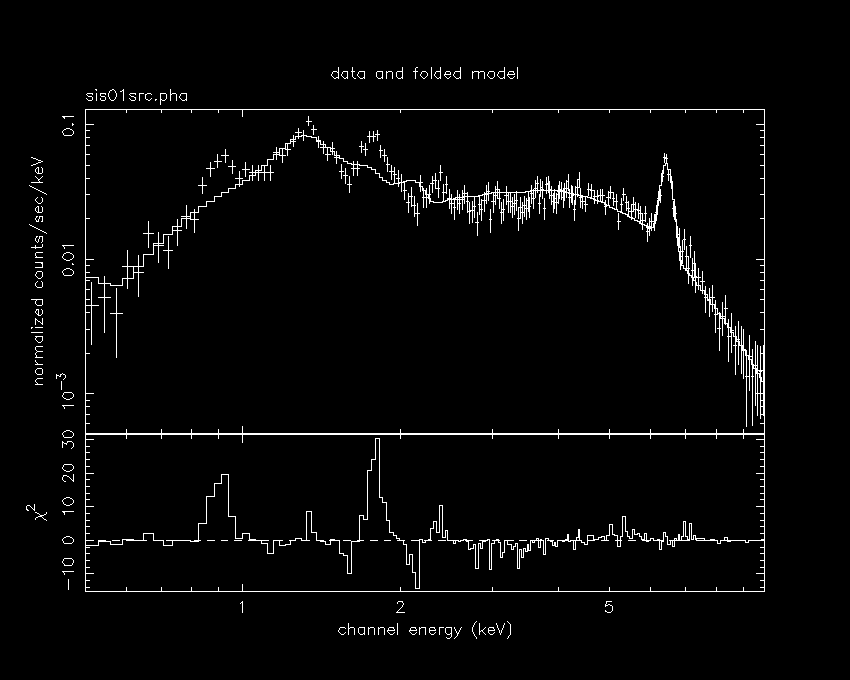
Note that the residual at the line energy ~ 1.3 keV has not yet disappeared,
it will do so only when we fit it properly by thawing (as opposed to
freezing) the line energy and line width parameters . Before that
we have to introduce the other three gauusian type emission lines at ~ 0.9,
1.8 and 2.4 keV. Therefore add the following components and give the inital
paramter values very carefully.
XSPEC>addcomp 5 ga
Input parameter value, delta, min, bot, top, and max values for ...
Current:         6.5      0.05         0         0     1E+06     1E+06
gaussian:LineE>0.9
Current:         0.1      0.05         0         0        10        20
gaussian:Sigma>0.1
Current:           1      0.01         0         0     1E+24     1E+24
gaussian:norm>0.0001
..
..
XSPEC>addcomp 6 ga
Input parameter value, delta, min, bot, top, and max values for ...
Current:         6.5      0.05         0         0     1E+06     1E+06
gaussian:LineE>1.8
Current:         0.1      0.05         0         0        10        20
gaussian:Sigma>0.1
Current:           1      0.01         0         0     1E+24     1E+24
gaussian:norm>0.0001
..
..
XSPEC>addcomp 7 ga
Input parameter value, delta, min, bot, top, and max values for ...
Current:         6.5      0.05         0         0     1E+06     1E+06
gaussian:LineE>2.4
Current:         0.1      0.05         0         0        10        20
gaussian:Sigma>0.1
Current:           1      0.01         0         0     1E+24     1E+24
gaussian:norm>1e-4
  ---------------------------------------------------------------------------
  ---------------------------------------------------------------------------
  Model:  wabs[1]( powerlaw[2] + gaussian[3] + gaussian[4] + gaussian[5] + gaussian[6] + gaussian[7] )
  Model Fit Model Component  Parameter  Unit     Value
  par   par comp
    1    1    1   wabs       nH       10^22      0.000     +/-  -1.000
    2    2    2   powerlaw   PhoIndex           0.1413     +/-  0.2287E-01
    3    3    2   powerlaw   norm               3.8363E-04 +/-  0.2075E-04
    4    4    3   gaussian   LineE    keV        6.441     +/-  0.8467E-02
    5    5    3   gaussian   Sigma    keV       9.7213E-02 +/-  0.1418E-01
    6    6    3   gaussian   norm               3.6545E-04 +/-  0.3623E-04
    7    7    4   gaussian   LineE    keV        1.300     frozen
    8    8    4   gaussian   Sigma    keV       0.1000     frozen
    9    9    4   gaussian   norm               6.9299E-05 +/-  0.1380E-04
   10   10    5   gaussian   LineE    keV       0.9000     +/-   0.000
   11   11    5   gaussian   Sigma    keV       0.1000     +/-   0.000
   12   12    5   gaussian   norm               1.0000E-04 +/-   0.000
   13   13    6   gaussian   LineE    keV        1.800     +/-   0.000
   14   14    6   gaussian   Sigma    keV       0.1000     +/-   0.000
   15   15    6   gaussian   norm               1.0000E-04 +/-   0.000
   16   16    7   gaussian   LineE    keV        2.400     +/-   0.000
   17   17    7   gaussian   Sigma    keV       0.1000     +/-   0.000
   18   18    7   gaussian   norm               1.0000E-04 +/-   0.000
  ---------------------------------------------------------------------------
  ---------------------------------------------------------------------------
 Chi-Squared =      616.4427     using   206 PHA bins.
 Reduced chi-squared =      3.244436     for    190 degrees of freedom
 Null hypothesis probability =  0.00
Now thaw the frozen line energy and line width of the gaussian at
1.3 keV
XSPEC>thaw 7 8
and fit.
XSPEC>fit
..
..
  ---------------------------------------------------------------------------
  ---------------------------------------------------------------------------
  Model:  wabs[1]( powerlaw[2] + gaussian[3] + gaussian[4] + gaussian[5] + gaussian[6] + gaussian[7] )
  Model Fit Model Component  Parameter  Unit     Value
  par   par comp
    1    1    1   wabs       nH       10^22     8.5170E-18 +/-  0.1058
    2    2    2   powerlaw   PhoIndex          -0.1886     +/-  0.5104E-01
    3    3    2   powerlaw   norm               2.3241E-04 +/-  0.3505E-04
    4    4    3   gaussian   LineE    keV        6.439     +/-  0.8420E-02
    5    5    3   gaussian   Sigma    keV       7.8779E-02 +/-  0.1646E-01
    6    6    3   gaussian   norm               3.3374E-04 +/-  0.3646E-04
    7    7    4   gaussian   LineE    keV        1.314     +/-  0.8657E-02
    8    8    4   gaussian   Sigma    keV       9.8008E-02 +/-  0.1612E-01
    9    9    4   gaussian   norm               1.1856E-04 +/-  0.2873E-04
   10   10    5   gaussian   LineE    keV       0.9165     +/-  0.1120E-01
   11   11    5   gaussian   Sigma    keV       6.8843E-02 +/-  0.3415E-01
   12   12    5   gaussian   norm               9.9507E-05 +/-  0.6356E-04
   13   13    6   gaussian   LineE    keV        1.811     +/-  0.8578E-02
   14   14    6   gaussian   Sigma    keV       6.6516E-02 +/-  0.1846E-01
   15   15    6   gaussian   norm               8.7201E-05 +/-  0.1890E-04
   16   16    7   gaussian   LineE    keV        2.368     +/-  0.1532E-01
   17   17    7   gaussian   Sigma    keV       3.8616E-02 +/-  0.4460E-01
   18   18    7   gaussian   norm               4.6904E-05 +/-  0.1705E-04
  ---------------------------------------------------------------------------
  ---------------------------------------------------------------------------
 Chi-Squared =      175.5206     using   206 PHA bins.
 Reduced chi-squared =     0.9336202     for    188 degrees of freedom
 Null hypothesis probability = 0.734
This is, again, one of the best fits that you can ever get. See the spectra
and the residual, it gives one of the best picture of emission lines superimposed
on the powerlaw continuum.
XSPEC>pl ld res
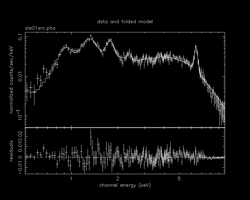
For better feel of the sepctra see the unfolded sepctra.
XSPEC>pl uf
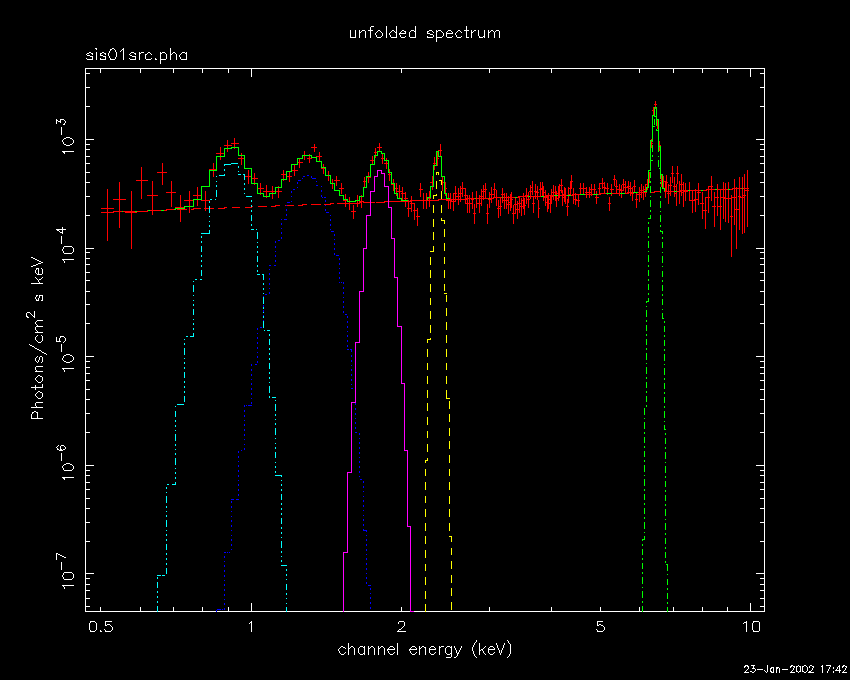
xspec also allows to view the unfolded spectra in terms of energy
per unit area per second per unit energy bin. Effectively it multiplies each
energy bin by its energy, note the unit of the y-axis.
XSPEC>pl euf
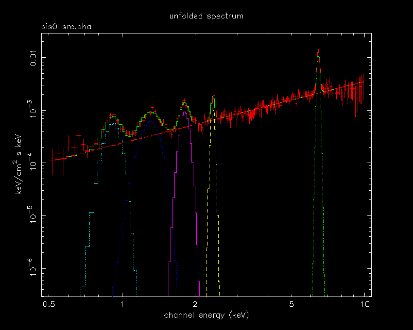
This brings us to the end of this exrecise. Lets quit xspec .
Before quitting you can also see the count rate sepctrum
XSPEC>pl count
XSPEC>quit
The eclipse spectrum that we have just analysed is remarkably
line dominated with a flat continuum. In addition to an intense 6.4 keV emission
line, which is due to fluorescence of iron in low ionization states, prominent
line features are obtained at 0.9, 1.3, 1.8, and 2.4 keV. These lines
are identified as the K-alpha
lines of He-like ions of neon, magnesium, silicon and sulfur. An eclipse spectrum
dominated by He-like K-alpha emission lines of heavy elements suggests that
radiative recombination followed by cascades is the dominant process in the
X-ray-irradiated stellar wind.
Our next exercise will be to fit cyclotron absorption line.
|


