Timing Analysis: Exercise 5
Effect of the orbital motion of the Pulsar - 1
Most X-ray pulsars are part of a binary system in which the source
of X-rays is moving around the common center of mass. Such orbital motion
should effect, by means of doppler effect, the periodic signal we are getting
from the pulsar. If we can detect the periodic changes in the pulse period
due to the doppler effect, we can use this information to determine the actual
orbital parameters of the binary system.
In this exercise we shall study the effect of the orbital motion on the
pulse period. We shall use a 3 day long light curve of pulsar
Cen X-3
, cenx-3_long.lc
, observed with RXTE. Basically we have to find the period in small consecutive
segments of the light curve. We shall use the task
efsearch
for this.
Invoke efsearch and provide various parameters as shown below. Please
enter all parameters exactly as shown because this exercise will take quite
long time.
pulsar> efsearch

efsearch 1.1 (xronos5.18)

Ser. 1 filename +options (or @file of filenames +options)[file1] cenx-3_long.lc
 Series 1 file   1:cenx-3_pca.lc

 Selected FITS extensions: 1 - RATE TABLE;

 Source ............ CEN_X-3             Start Time (d) .... 10507 00:19:27.562
 FITS Extension ....  1 - `RATE      `   Stop Time (d) ..... 10510 19:57:03.562
 No. of Rows .......      1873744        Bin Time (s) ......   0.1250
 Right Ascension ... 1.70313293E+02      Internal time sys.. Converted to TJD
 Declination ....... -6.06232986E+01     Experiment ........ XTE      PCA

 Corrections applied: Vignetting - No ; Deadtime - No ; Bkgd - No ; Clock - Yes
 Selected Columns:  1- Time;  2- Y-axis;  3- Y-error;  4- Fractional exposure;

 File contains binned data.

Name of the window file ('-' for default window)[-] -

 Expected Start ... 10507.01351345407  (days)       0:19:27:562  (h:m:s:ms)
 Expected Stop .... 10510.83129123185  (days)      19:57: 3:562  (h:m:s:ms)

 Default Epoch is:  10507.00000
Type INDEF to accept the default value
 Epoch format is days.
Epoch[34 234.23] 10507.00000
 Period format is seconds.
Period[88.87] 4.81
Period derivative [0] 0
 Expected Cycles ..          68577.13
 Default phase bins per period are:         8
 Type INDEF to accept the default value
Phasebins/Period {value or neg. power of 2}[-3] 16

 Newbin Time ......    0.30062500      (s)
 Maximum Newbin No.           1097235

 Default Newbins per Interval are:     1097235
 (giving       1 Interval of      1097235 Newbins)
 Type INDEF to accept the default value

Number of Newbins/Interval[10] 20000
 Maximum of      55 Intvs. with        20000 Newbins of      0.300625     (s)
 Default resolution is 0.1924000000E-02
 Type INDEF to accept the default value
So far we have taken all available newbins in one interval in order to determine
period over entire light curve. However, here we take only 20000 newbins
per interval i.e. we devide the light curve in 55 segments and calculate
period over each segment seperately.
Resolution for period search {value or neg. power of 2}[.03] 0.0001
 Default number of periods is       128
 Type INDEF to accept the default value
Number of periods to search[100] 1024

Name of output file[default]
Do you want to plot your results?[yes]
Enter PGPLOT device[/XW]

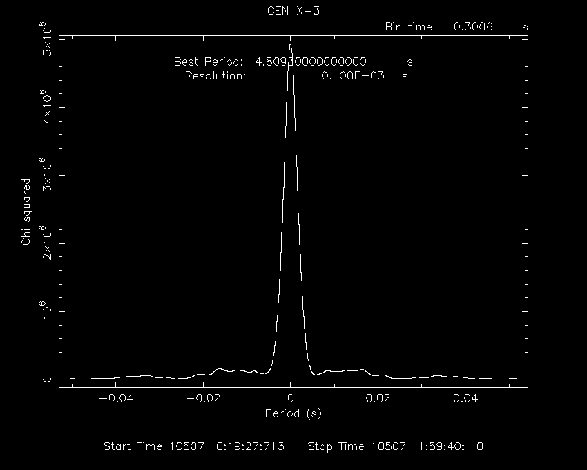
    1024 analysis results per interval

This will take quite long time. Once calculation of one interval is over, it
will show the result for that interval. Please note down the start and stop
time(hh:mm:ss), shown below the x-axis and the best period (with 4 digits
after decimal). After quiting from the PLT> prompt, calculation for the
next interval will proceed and result for that interval will be shown. Again
note down the start / stop time and best period. This will continue till 100
% calculation is over. Period search for each interval will take about
one minute i.e. the entire exercise will take about one hour.
Now you should have a list of start and stop for each interval and the
pulse period during that interval. Find out the average of the start and
stop times of each interval and create a file having two column, mid-time
for each interval and pulse period during that period. Use 24 hour format
for time and for next day time add 24 hour so that time is continuously increasing.
It will be even better if you convert time in mimutes or seconds from the
start time of the first interval.
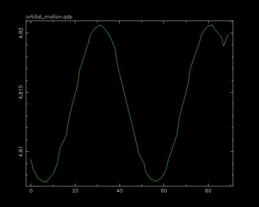
You can plot this file with QDP to see the changes in the pulse period
with time due the orbital motion. QDP is a general purpose plotting program
to plot files containing ASCII data. QDP also uses the same PLT plotting
routine which you have been using so far. Invoke QDP as shown below.
pulsar> qdp filename
 To produce plot, please enter
PGPLOT file/type:/xw
PLT>

You should see the periodic change in the pulse period. When the period
is smaller i.e. frequeency is higher, the pulser is approaching us, and when
period is larger the pulsar is receding away from us. Details of this plot
such as the shape of the curve, difference of maximum and minimum period etc.
gives us information about the geometry of the binary orbit.
|


