Timing Analysis: Exercise 2
Finding period by Fourrier analysis
In the previous exercise we saw the individual pulses in the light curve
of Cen X-3
. In this exercise we shall generate a Power Density Spectrum (PDS)
from this light curve in order to find out its pulse period. The XRONOS
package has a task named
powspec
, which generates the Fourier spectrum or PDS of a light curve. You already
have the light curve file cenx-3_pca.lc
in your directory. Invoke powspec by entering the command at the
prompt and give answers to the queries as shown below.
pulsar> powspec

powspec 1.0 (xronos5.18)

Ser. 1 filename +options (or @file of filenames +options)[file1] cenx-3_pca.lc
 Series 1 file   1:cenx-3.lc

 Selected FITS extensions: 1 - RATE TABLE;

 Source ............ CEN_X-3             Start Time (d) .... 10507 00:19:27.562
 FITS Extension ....  1 - `RATE      `   Stop Time (d) ..... 10507 00:21:32.562
 No. of Rows .......         1000        Bin Time (s) ......   0.1250
 Right Ascension ...                     Internal time sys.. Literal
 Declination .......                     Experiment ........

 Corrections applied: Vignetting - Yes; Deadtime - Yes; Bkgd - Yes; Clock - Yes
             values: 1.00000000       1.00000000       1.00000000

 Selected Columns:  1- Time;  3- Y-axis;  4- Y-error;  5- Fractional exposure;

 File contains binned data.

Name of the window file ('-' for default window)[-] -
 Expected Start ... 10507.01351345407  (days)       0:19:27:562  (h:m:s:ms)
 Expected Stop .... 10507.01496021276  (days)       0:21:32:562  (h:m:s:ms)

 **** Warning: Newbin Time must be an integer multiple of Minimum Newbin Time
 Minimum Newbin Time   0.12500000      (s)
 for Maximum Newbin No..             60000

 Default Newbin Time is:  1.0000000    (s) (to have 1 Intv. of    8192 Newbins)
 Type INDEF to accept the default value

Newbin Time or negative rebinning[4.6692607009327] 0.125
All the queries so far are similar to those of lcurve! You give the name
of the light curve file, window file (which is default in our case)
and new bin time. Notice the warning saying that "Newbin Time must be an
integer multiple of Minimum Newbin Time". This is a requirement of powspec.
 Newbin Time ......    0.12500000      (s)
 Maximum Newbin No.              60000

 Default Newbins per Interval are:        8192
 (giving       8 Intervals of         8192 Newbins)
 Type INDEF to accept the default value

Number of Newbins/Interval[10] 8192
 Maximum of       8 Intvs. with         8192 Newbins of      0.125000     (s)
There is one more requirement of powspec, that total number of newbins
per interval should be an integer power of 2. Here we shall accept
the default 8192 newbins per interval. This will give total 8 intervals i.e.
the analysis will be carried out on 8 independent segments of the light curve
each of 8192 bins. However, since total number of newbins are not multiple
of 8192, the last segment will be half empty and we shall use only first 7
full segments.
Default intervals per frame are:         1
Type INDEF to accept the default value
Number of Intervals/Frame[1] 7
 Results from up to       7 Intvs. will be averaged in a Frame
A frame is made by averaging results of the analysis of one or more contiguous
intervals. Here we average 7 intervals in one frame and discard the last
interval. such averaging helps particularly in improving the statistics.
Rebin results? (>1 const rebin, <-1 geom. rebin, 0 none)[0] 0
Right now we are not rebining our result. However, later you can experiment
here by giving 1.01, 1.03, 1.05 and similar negative values as rebinning
factor and see the effect.
Name of output file[default] test
Do you want to plot your results?[yes] yes
Enter PGPLOT device[/XW] /xw

    4096 analysis results per interval

 13% completed
 Intv    1   Start 10507  0:19:27
 Ser.1     Avg  1006.        Chisq 0.3487E+06   Var 0.3427E+06 Newbs.   8192
           Min  248.0          Max  3704.    expVar  8050.      Bins   8192
Power spectrum ready !
 Intv    2   Start 10507  0:36:31
 Ser.1     Avg  1892.        Chisq 0.8259E+06   Var 0.1526E+07 Newbs.   8192
           Min  416.0          Max  8544.    expVar 0.1514E+05  Bins   8192
Power spectrum ready !
 Intv    3   Start 10507  0:53:35
 Ser.1     Avg  2701.        Chisq 0.1234E+07   Var 0.3254E+07 Newbs.   8192
           Min  544.0          Max 0.1116E+05expVar 0.2160E+05  Bins   8192
Power spectrum ready !
 Intv    4   Start 10507  1:10:39
 Ser.1     Avg  3868.        Chisq 0.1730E+07   Var 0.6535E+07 Newbs.   8192
           Min  672.0          Max 0.1471E+05expVar 0.3094E+05  Bins   8192
Power spectrum ready !
 Intv    5   Start 10507  1:27:43
 Ser.1     Avg  4722.        Chisq 0.1111E+07   Var 0.8197E+07 Newbs.   5120
           Min  1176.          Max 0.1633E+05expVar 0.3778E+05  Bins   5120
Power spectrum ready !
 Intv    6   Start 10507  1:54:23
 Ser.1     Avg  4806.        Chisq 0.2097E+07   Var 0.9842E+07 Newbs.   8192
           Min  944.0          Max 0.1780E+05expVar 0.3845E+05  Bins   8192
Power spectrum ready !
 Intv    7   Start 10507  2:11:27
 Ser.1     Avg  4696.        Chisq 0.1486E+07   Var 0.8946E+07 Newbs.   6240
           Min  928.0          Max 0.2020E+05expVar 0.3757E+05  Bins   6240
Power spectrum ready !
PLT>
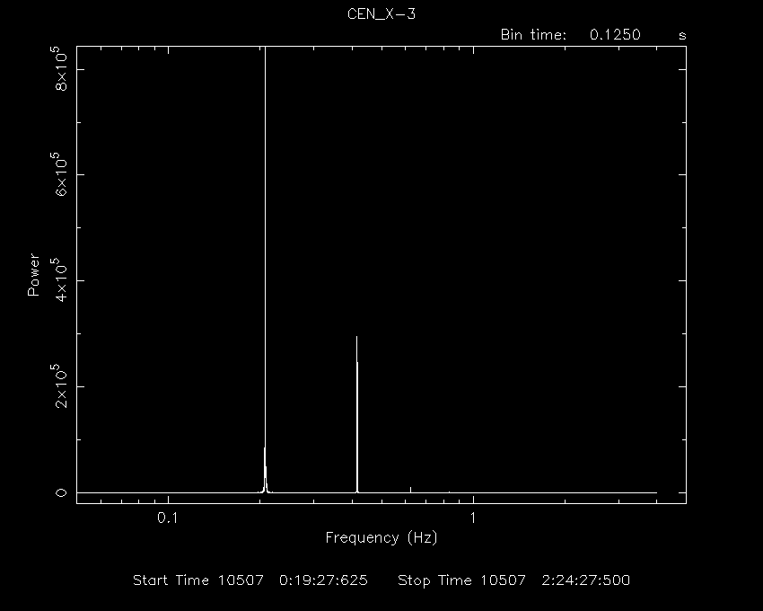
Now you should see a Power Density Spectrum with two clear peaks. The prominent
peak corresponds to the pulse period whereas the second peak corresponds
to the first harmonic of the period.
You can resize and plot the X axis logarithmically by executing a PLT
command. This will help to find out the exact position of the peak corresponding
to pulse period.
PLT> r x 0.05 5
PLT> log x on
PLT> plot
You should see a plot as shown below.

You can also find out the exact frequency of the peak by fitting a function
like gaussian to the peak. Consult the QDP/PLT User's Guide or one of the
instructors to find out how to do this.
|


