Timing Analysis: Exercise 6
Effect of the orbital motion of the Pulsar - 2
In the previous exercise we studied the doppler shift in pulsar period due
to its orbital motion. The same phemenomenon can also lead to one more interesting
effect, namely, variation in the pulse arrival time. When the pulsar is nearest
to us pulses arrive earlier and when the pulsar is farthest pulses arrive
later. If we can precisely measure the arrival time difference then we can
obtain more accurate information about the geometry of the binary orbit.
What is done in the pulse arrival time analysis is to fold small segments
of a long light curve with accurately measured average pulse period. In this
exercise we shall follow the same procedure with same light curve of
X-ray pulsar Cen X-3 which we used in the previous exercise. The XRONOS task
we shall be using, as you shoud know by now, is
efold
.
Invoke efold and provide all parameters exactly as shown below. Enter
period with all digits shown after decimal i.e. period accurate upto micro
second.
pulsar> efold

efold 1.1 (xronos5.18)

Number of time series for this task[1]
Ser. 1 filename +options (or @file of filenames +options)[file1] cenx-3_long.lc
 Series 1 file   1:cenx-3_pca.lc

 Selected FITS extensions: 1 - RATE TABLE;

 Source ............ CEN_X-3             Start Time (d) .... 10507 00:19:27.562
 FITS Extension ....  1 - `RATE      `   Stop Time (d) ..... 10510 19:57:03.562
 No. of Rows .......      1873744        Bin Time (s) ......   0.1250
 Right Ascension ... 1.70313293E+02      Internal time sys.. Converted to TJD
 Declination ....... -6.06232986E+01     Experiment ........ XTE      PCA

 Corrections applied: Vignetting - No ; Deadtime - No ; Bkgd - No ; Clock - Yes
 Selected Columns:  1- Time;  2- Y-axis;  3- Y-error;  4- Fractional exposure;

 File contains binned data.

Name of the window file ('-' for default window)[-] -

 Expected Start ... 10507.01351345407  (days)       0:19:27:562  (h:m:s:ms)
 Expected Stop .... 10510.83129123185  (days)      19:57: 3:562  (h:m:s:ms)

 Default Epoch is:  10507.00000
Type INDEF to accept the default value
 Epoch format is days.
Epoch[34 234.23] 10507.00000
 Period format is seconds.
Period[88.87] 4.8144045
Period derivative         [0] 0
 Expected Cycles ..          68514.39
 Default phase bins per period are:        10
 Type INDEF to accept the default value
Phasebins/Period {value or neg. power of 2}[-3] 32

 Newbin Time ......    0.15045014      (s)
 Maximum Newbin No.           2192461

 Default Newbins per Interval are:     2192461
 (giving       1 Interval of      2192461 Newbins)
 Type INDEF to accept the default value

Number of Newbins/Interval[10] 5000
 Maximum of     439 Intvs. with         5000 Newbins of      0.150450     (s)
Default intervals per frame are:       439
Type INDEF to accept the default value
Number of Intervals/Frame[1] 1
 Results from up to       1 Intvs. will be averaged in a Frame
Here we have folded small segments (5000 newbins) of the entire light
curve and observing each interval seperately
Name of output file[default]
Do you want to plot your results?[yes]
Enter PGPLOT device[/XW]

      32 analysis results per interval

 Intv    1   Start 10507  0:19:27
     Ser.1     Avg  967.7        Chisq 0.1712E+06   Var 0.2198E+06 Newbs.     32
               Min  469.0          Max  1866.    expVar  41.14      Bins   6018
 Folded light curve ready
PLT> q
Writing output file: cenx-3_pca.fef
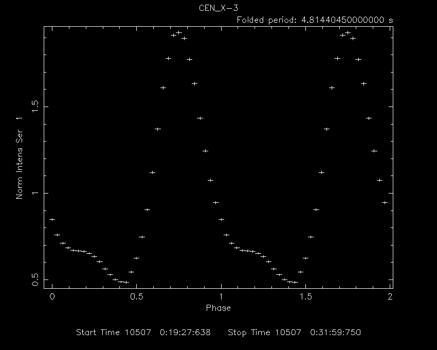
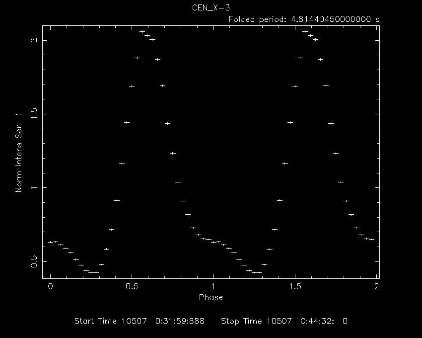
Result of first interval will be shown as above. Note down the phase
of the peak in the pulse profile. Analysis for other intervals will
continue after quiting from the PLT> and result of the next interval will
shown as below. Again note down the peak phase. Notice the decrease in the
phase i.e. left wards shift of the pulse profile. In other words the pulsar
is approaching us and pulses are arriving earlier. Pulse peak phase will keep
on decreasing for some intervals and then slowly it will increasing i.e.
the pulsar start to move away from us. To notice this, you will need to go
thourgh at least first 100 or so intervals.
In the present exercise we have just noticed the change in pulse arrival
time due to the orbital motion. In actual practise, this process is little
more involved. First one has to obtain average pulse profile and then find
out exact arrival time difference for each interval by cross-correlating
the pulse profile in that interval with the average profile. From the exact
time difference and absolute time of each interval one can obtain geometry
of the binary orbit.
|