1st ASTROSAT Workshop - Pulsar Astrophysics

Spectral Analysis: Exercise 2

Observation of strong iron line in X-ray Pulsar GX 1+4

This exercise will give you further practice of spectral fitting, introducing the emission line along with the continuum components. Here we will analyse the sepctra of pulsar GX 1+4 observed with GIS (Gas Imaging Spectrometer) instrument onboard ASCA satellite. First copy the required source and background spectrum files and response files, gx1+4_gis2src.pha , gx1+4_gis2bkg.pha , gis2.rmf and gis2.arf . Lets start with the good old xspec .

pulsar> xspec

and specify the source data (PHA) file, response matrix file, .arf file and the background noise file.

XSPEC>da gis2src.pha
Net count rate (cts/s) for file   1   1.077    +/-  5.2096E-03
   1 data set is in use
XSPEC>resp gis2.rmf
XSPEC>arf gis2.arf
XSPEC>back gis2bkg.pha
 Net count rate (cts/s) for file   1  0.9829    +/-  5.3140E-03( 91.3% total)
   using response (RMF) file...       gis2.rmf
   using auxiliary (ARF) file...      gis2.arf
   using background file...           gis2bkg.pha

Set the plotting device and the change unit of x-axis to energy (keV).

XSPEC>cpd /xw
XSPEC>setp ener

And type plot data and pl ld to see the spectra. Decide that (rather in this case we decide for you) data below 0.7 keV and above 10.0 keV need to be ignored.

XSPEC>ig **-0.7 10.0-**
XSPEC>pl

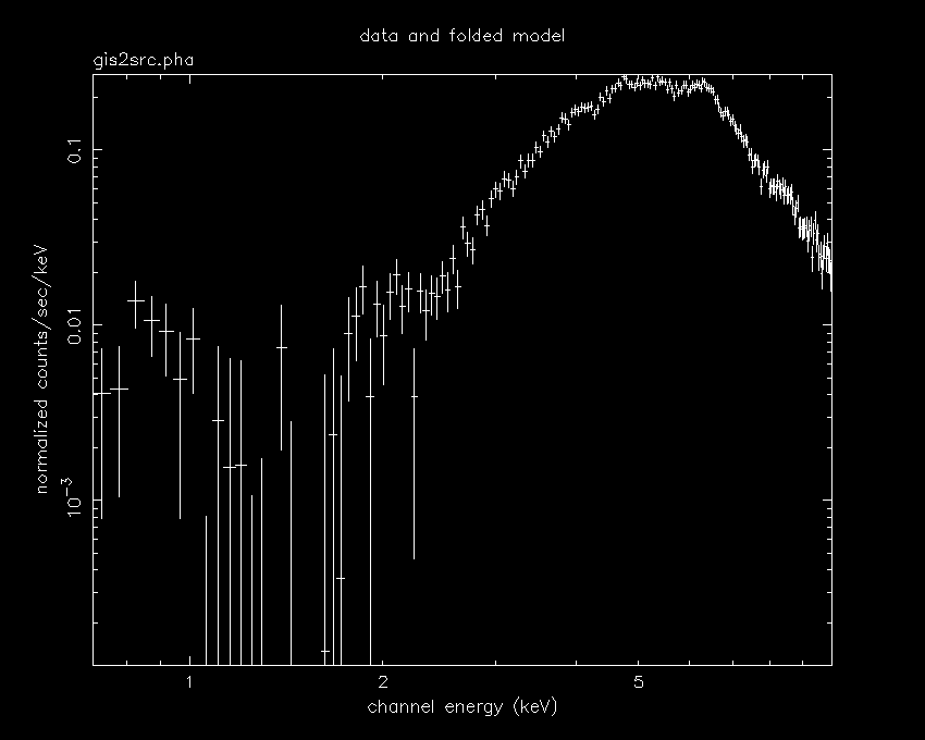
This is the spectrum you see.

spectra of GX 1+4

Now lets commence to fit this innocous looking spectra. As usual, lets start with the standard and omnipresent powerlaw model.

XSPEC>mo pow
  Model:  powerlaw[1]
Input parameter value, delta, min, bot, top, and max values for ...
Current:           1      0.01        -3        -2         9        10
powerlaw:PhoIndex>
Current:           1      0.01         0         0     1E+24     1E+24
powerlaw:norm>
  ---------------------------------------------------------------------------
  ---------------------------------------------------------------------------
  Model:  powerlaw[1]
  Model Fit Model Component  Parameter  Unit     Value
  par   par comp
    1    1    1   powerlaw   PhoIndex            1.000     +/-   0.000
    2    2    1   powerlaw   norm                1.000     +/-   0.000
  ---------------------------------------------------------------------------
  ---------------------------------------------------------------------------
 Chi-Squared =     3.3933906E+09 using   197 PHA bins.
 Reduced chi-squared =     1.7402004E+07 for    195 degrees of freedom
 Null hypothesis probability =  0.00
XSPEC>pl
XSPEC>fit
 Chi-Squared    Lvl  Fit param # 1     2
   14310.6     -1     -2.383      3.2649E-05
   11301.2     -1     -2.154      4.3365E-05
   10258.5     -1     -1.970      6.7552E-05
   8191.41     -2     -1.368      2.1001E-04
   8155.36     -1     -1.371      1.8771E-04
   8098.40     -2     -1.416      1.7777E-04
   8090.04     -1     -1.417      1.8513E-04
   8082.10     -2     -1.403      1.8785E-04
   8081.38     -1     -1.403      1.8578E-04
   8080.77     -2     -1.406      1.8511E-04
 Number of trials exceeded - last iteration delta =   0.6108
 Continue fitting? (Y)
..

Continue till the least chi-square value is reached.

..
  ---------------------------------------------------------------------------
  ---------------------------------------------------------------------------
  Model:  powerlaw[1]
  Model Fit Model Component  Parameter  Unit     Value
  par   par comp
    1    1    1   powerlaw   PhoIndex           -1.405     +/-  0.1369E-01
    2    2    1   powerlaw   norm               1.8569E-04 +/-  0.8896E-05
  ---------------------------------------------------------------------------
  ---------------------------------------------------------------------------
 Chi-Squared =      8080.686     using   197 PHA bins.
 Reduced chi-squared =      41.43941     for    195 degrees of freedom
 Null hypothesis probability =  0.00

The best fit chi-square (and reduced chi-square) is extremely poor. See the best fit model with residual (typing pl ld res). As is always the case, we have to add an absorption component (wabs or phabs ) for absortpion due to effective Hydrogen column in the direction of the source

XSPEC>addcomp 1 wabs
Input parameter value, delta, min, bot, top, and max values for ...
Current:           1     0.001         0         0     1E+05     1E+06
wabs:nH>
  ---------------------------------------------------------------------------
  ---------------------------------------------------------------------------
  Model:  wabs[1]( powerlaw[2] )
  Model Fit Model Component  Parameter  Unit     Value
  par   par comp
    1    3    1   wabs       nH       10^22      1.000     +/-   0.000
    2    1    2   powerlaw   PhoIndex           -1.405     +/-  0.1370E-01
    3    2    2   powerlaw   norm               1.8575E-04 +/-  0.8897E-05
  ---------------------------------------------------------------------------
  ---------------------------------------------------------------------------
 Chi-Squared =      7300.136     using   197 PHA bins.
 Reduced chi-squared =      37.62957     for    194 degrees of freedom
 Null hypothesis probability =  0.00

and fit.

XSPEC>fit
..
..
  ---------------------------------------------------------------------------
  ---------------------------------------------------------------------------
  Model:  wabs[1]( powerlaw[2] )
  Model Fit Model Component  Parameter  Unit     Value
  par   par comp
    1    3    1   wabs       nH       10^22      21.72     +/-  0.4086
    2    1    2   powerlaw   PhoIndex            1.342     +/-  0.4250E-01
    3    2    2   powerlaw   norm               6.3922E-02 +/-  0.5426E-02
  ---------------------------------------------------------------------------
  ---------------------------------------------------------------------------
 Chi-Squared =      456.1984     using   197 PHA bins.
 Reduced chi-squared =      2.351538     for    194 degrees of freedom
 Null hypothesis probability = 3.599E-23

The model has improved considerably, but still is not acceptable. Observe the spectrum, best fit model and its residual.

XSPEC>pl ld delchi

Observe the excess between 6-7 keV.

spectra of GX 1+4

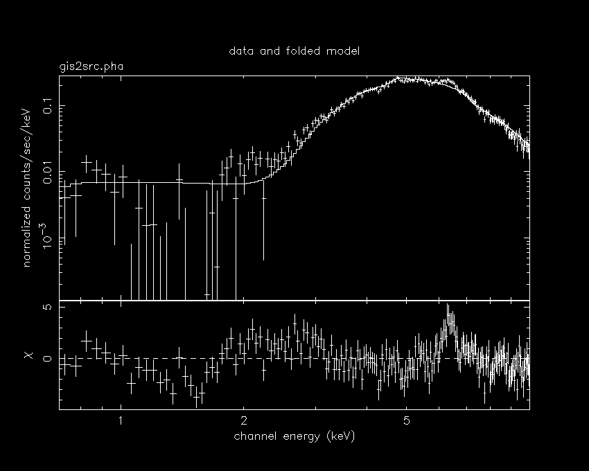
The keyword delchi plots the residuals in terms of sigmas with error bars of size one. The residual in the low energy region (less than 2 keV) is due to relatively poor quality data, whereas the excess between 6-7 keV is due to Fe emission line. Therefore add gaussian line component to the model.

XSPEC>addcomp 3 ga
Input parameter value, delta, min, bot, top, and max values for ...
Current:         6.5      0.05         0         0     1E+06     1E+06
gaussian:LineE>
Current:         0.1      0.05         0         0        10        20
gaussian:Sigma>
Current:           1      0.01         0         0     1E+24     1E+24
gaussian:norm>
  ---------------------------------------------------------------------------
  ---------------------------------------------------------------------------
  Model:  wabs[1]( powerlaw[2] ) + gaussian[3]
  Model Fit Model Component  Parameter  Unit     Value
  par   par comp
    1    3    1   wabs       nH       10^22      21.73     +/-  0.4090
    2    1    2   powerlaw   PhoIndex            1.342     +/-  0.4253E-01
    3    2    2   powerlaw   norm               6.3927E-02 +/-  0.5438E-02
    4    4    3   gaussian   LineE    keV        6.500     +/-   0.000
    5    5    3   gaussian   Sigma    keV       0.1000     +/-   0.000
    6    6    3   gaussian   norm                1.000     +/-   0.000
  ---------------------------------------------------------------------------
  ---------------------------------------------------------------------------
 Chi-Squared =     5.6398118E+08 using   197 PHA bins.
 Reduced chi-squared =      2952781.     for    191 degrees of freedom
 Null hypothesis probability =  0.00

This absurd value of chi-square is due to the arbitrary initial value of the gaussian line parameters that we have input. Just fit the data and see the fun.

XSPEC>fit
..
..
---------------------------------------------------------------------------
  ---------------------------------------------------------------------------
  Model:  wabs[1]( powerlaw[2] ) + gaussian[3]
  Model Fit Model Component  Parameter  Unit     Value
  par   par comp
    1    3    1   wabs       nH       10^22      19.72     +/-  0.4490
    2    1    2   powerlaw   PhoIndex            1.274     +/-  0.4744E-01
    3    2    2   powerlaw   norm               4.9797E-02 +/-  0.4770E-02
    4    4    3   gaussian   LineE    keV        6.436     +/-  0.4277E-01
    5    5    3   gaussian   Sigma    keV       0.4722     +/-  0.5708E-01
    6    6    3   gaussian   norm               1.0815E-03 +/-  0.2245E-03
  ---------------------------------------------------------------------------
  ---------------------------------------------------------------------------
 Chi-Squared =      292.3154     using   197 PHA bins.
 Reduced chi-squared =      1.530447     for    191 degrees of freedom
 Null hypothesis probability = 3.261E-06

This is a good fit, maybe not as good as the one in the previous exercise, because the data available in the low energy range is not excellent. Plot the spectra, best fit model and the residual.

XSPEC>pl ld chi

chi is another keyword of the plot command which gives the chi-square contribution of each energy bin.

spectra of GX 1+4

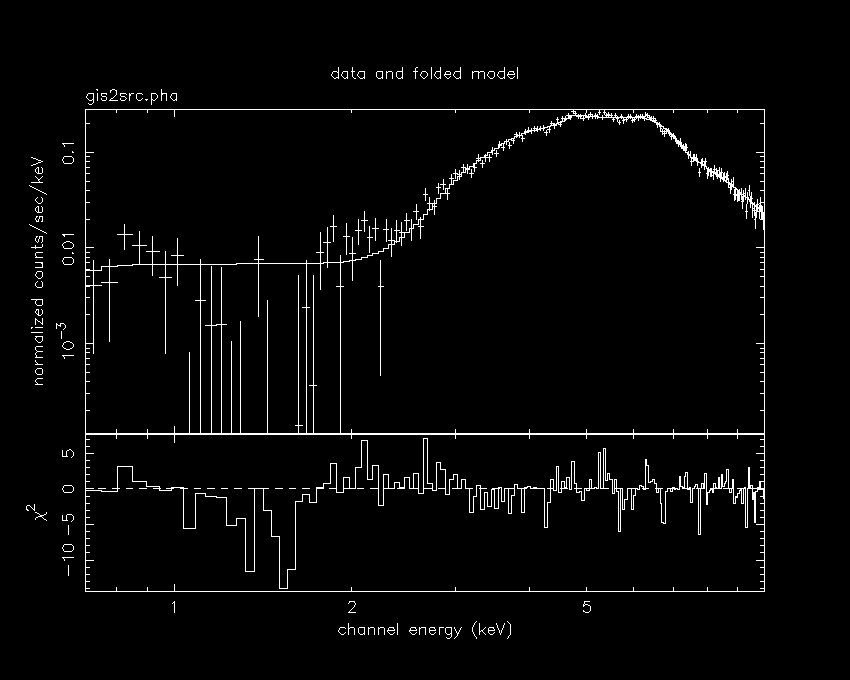
Now you can see that the contribution to chi-square is mainly from the region <2 keV. Most importantly, the excess between 6-7 keV is no longer present, vindicating our supposition of the presence of Fe emission line.
You may plot the unfolded spectra.

XSPEC>pl uf

spectra of GX 1+4

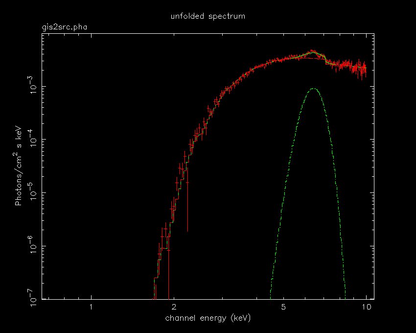
It is possible to see the individual model components in the folded spectra also.

XSPEC>setp add

To check for other keywords for setplot you type help setpl, in fact you will get help for every command by typing help followed by the command name. Typing only help will give a list of all the commands of xspec.

XSPEC>pl ld chi

You can see that you need to adjust the scale of the y axis of the sepctrum to get a proper figure of the folded spectra along with the individual model components. Type iplot, this command starts the QDP/PLT subroutine. QDP (quick and dandy plotter) is a program used for all the front end plotting program for FTOOLS and XANADU. Once you get the PLT prompt you can set the range of the y-axis as per the following syntax. You may browse through the main commands of QDP/PLT and their usage by the help command while in the PLT prompt.

XSPEC>iplot
PLT>r y .001
PLT>pl

spectra of GX 1+4

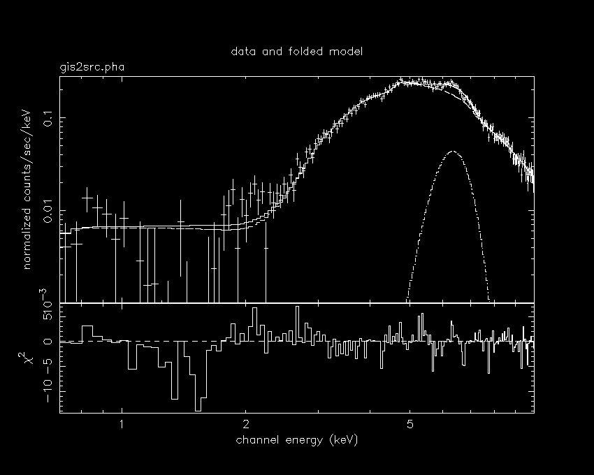
Notice the Fe emission line among the continuum components (powerlaw ).
You can quit QDP/PLT anytime by typing quit and you will come back to xspec. Lets quit the package and get on with the next exercise.

PLT>quit

You can also see the number of X-ray photons detected in each energy channel

xspec>pl counts

xspec>quit

The hydrogen column density towards this source that we have derived is very high. Though this source is in the galactic plane, the measured column density is much larger than the average galactic hydgoren column density in this direction of the sky. This indicates that most of the absorbing material is very close to the source, probably circumstellar material. A further evidence for this is that the column density is found to vary significantly with time, which must be related to the level of activity of the companion star. The centre of the gaussian line profile is ~6.4 keV. This indicates that the absorbing material, which also gives rise to the iron K-alpha fluorescence emission is relative cold and not very highly ionised.

Our next exercise will be to fit more than one emission line.

This workshop is being organized by Department of Astronomy & Astrophysics, Tata Institute of Fundamental Research (TIFR) and is sponsored by Indian Space Research Organization (ISRO).