Timing Analysis: Exercise 3
Finding period by Epoch folding
In second exercise we have obtained the pulse period for X-ray pulsar Cen
X-3 from its power density spectrum. In this exercise we shall determine the
pulse period for the same source using light curve folding method. This method
is very useful to find out accurate period if an approximate period is known.
The XRONOS package has a task named
efsearch
which folds the light curve with large number of periods around the approximate
period and finds the best period by chi square maximization. For this exercise
also we shall use the same light curve cenx-3_pca.lc
, which we used in the last exercise.
Invoke efsearch by entering the command at the prompt and
answer the queries as usual.
pulsar> efsearch

efsearch 1.1 (xronos5.18)

Ser. 1 filename +options (or @file of filenames +options)[cenx-3.lc]cenx-3_pca.lc
 Series 1 file   1:cenx-3.lc

 Selected FITS extensions: 1 - RATE TABLE;

 Source ............ CEN_X-3             Start Time (d) .... 10507 00:19:27.562
 FITS Extension ....  1 - `RATE      `   Stop Time (d) ..... 10507 02:24:27.559
 No. of Rows .......        60000        Bin Time (s)......    0.1250
 Right Ascension ...                     Internal time sys.. Literal
 Declination .......                     Experiment ........

 Corrections applied: Vignetting - Yes; Deadtime - Yes; Bkgd - Yes; Clock - Yes
             values: 1.00000000       1.00000000       1.00000000

 Selected Columns:  1- Time;  3- Y-axis;  4- Y-error;  5- Fractional exposure;

 File contains binned data.

Name of the window file ('-' for default window)[-] -

 Expected Start ... 10507.01351345407  (days)       0:19:27:562  (h:m:s:ms)
 Expected Stop .... 10507.10031897535  (days)       2:24:27:559  (h:m:s:ms)

 Default Epoch is:  10507.00000
Type INDEF to accept the default value
 Epoch format is days.
Epoch[10507.00000] 10507.00000
 Period format is seconds.
Period[5.0] 4.8
Period derivative       [0] 0
 Expected Cycles ..           1562.50
Epoch is the reference point with respect to the what the light curve
is folded. Here we accept the default value, which is the starting point
of the light curve. We give the approximate period (obtained using power
dinsity spectrum?) and the period derivative or the change in period with
time, which, in our case is zero.
 Default phase bins per period are:         8
 Type INDEF to accept the default value
Phasebins/Period {value or neg. power of 2}[16] 16

 Newbin Time ......    0.30000000      (s)
 Maximum Newbin No.             25000

 Default Newbins per Interval are:       25000
 (giving       1 Interval of        25000 Newbins)
 Type INDEF to accept the default value

Number of Newbins/Interval[25000] 25000
 Maximum of       1 Intvs. with        25000 Newbins of      0.300000     (s)
Here we devide each pulse in 16 phases i.e. each newbin will be one sixteenth
of the pulse period or 0.3 seconds. We take all available newbins in the
same interval.
 Default resolution is 0.1536000000E-02
 Type INDEF to accept the default value
Resolution for period search {value or neg. power of 2}[0.01] 0.0001
 Default number of periods is       128
 Type INDEF to accept the default value
Number of periods to search[4096] 4096
Here we specify total number of periods and resolution for the period search.
We are asking it to fold the light curve with 4096 different period seperated
by 0.1 milli-second around the approximate period of 4.8 seconds.
Name of output file[default]
Do you want to plot your results?[yes]
Enter PGPLOT device[/XW]
4096 analysis results per interval
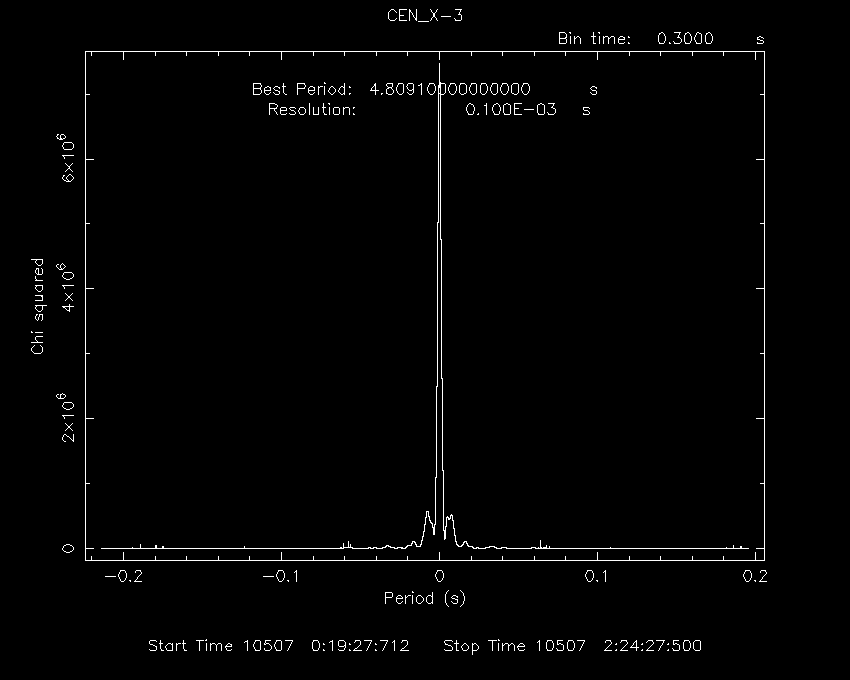
Chisq. vs. period ready
Period : 4.809 dP/dt : 0.000
Intv 1 Start 10507 0:19:27
Ser.1 Avg 3257. Chisq 0.7471E+07 Var 0.3719E+07 Newbs.
16 Min 1177. Max 7050. expVar 7.966 Bins
52320
PLT>
Now you should see the following plot of chi-square vs. period. The plot
also gives the best period.
You can play around various parameters to see their effect on the final
result.
The task efsearch gives you only best period, but it does not show
the folded pulse profile.
To get the folded pulse profile, XRONOS has another taks called
efold
.
Invoke efold and answer the queries as usual by giving the default
epoch, exact period obtained with efsearch, 16 phase bins and take
all newbins in one interval.
pulsar> efold
efold 1.1 (xronos5.18)
Number of time series for this task[1]
Ser. 1 filename +options (or @file of filenames +options)[cenx-3.lc] cenx-3.lc
Series 1 file 1:cenx-3.lc
Selected FITS extensions: 1 - RATE TABLE;
Source ............ CEN_X-3 Start Time (d) .... 10507 00:19:27.562
FITS Extension .... 1 - `RATE ` Stop Time (d) ..... 10507 02:24:27.559
No. of Rows ....... 60000 Bin Time (s) ...... 0.1250
Right Ascension ... Internal time sys.. Literal
Declination ....... Experiment ........
Corrections applied: Vignetting - Yes; Deadtime - Yes; Bkgd - Yes; Clock - Yes
values: 1.00000000 1.00000000 1.00000000
Selected Columns: 1- Time; 3- Y-axis; 4- Y-error; 5- Fractional exposure;
File contains binned data.
Name of the window file ('-' for default window)[-] -
Expected Start ... 10507.01351345407 (days) 0:19:27:562 (h:m:s:ms)
Expected Stop .... 10507.10031897535 (days) 2:24:27:559 (h:m:s:ms)
Default Epoch is: 10507.00000
Type INDEF to accept the default value
Epoch format is days.
Epoch[10507.00000] 10507.00000
Period format is seconds.
Period[4.812] 4.8091
Expected Cycles .. 1559.54
Default phase bins per period are: 10
Type INDEF to accept the default value
Phasebins/Period {value or neg. power of 2}[16] 16
Newbin Time ...... 0.30056875 (s)
Maximum Newbin No. 24953
Default Newbins per Interval are: 24953
(giving 1 Interval of 24953 Newbins)
Type INDEF to accept the default value
Number of Newbins/Interval[416] 24953
Maximum of 1 Intvs. with 24953 Newbins of 0.300569 (s)
Default intervals per frame are: 1
Type INDEF to accept the default value
Number of Intervals/Frame[1] 1
Results from up to 1 Intvs. will be averaged in a Frame
Name of output file[test]
Do you want to plot your results?[yes]
Enter PGPLOT device[/xw]
16 analysis results per interval
87% completed
Intv 1 Start 10507 0:19:27
Ser.1 Avg 3257. Chisq 0.7471E+07 Var 0.3719E+07 Newbs. 16
Min 1177. Max 7050. expVar 7.966 Bins 52320
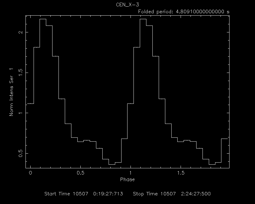
Folded light curve ready
PLT>
PLT> line step
PLT> plot
PLT> quit
Now you should see the following figure showing the folded pulse profile.
|